Add-ons and more

Profiling: using kernprof in Blender add-ons

When implementing add-ons that contain very time consuming activities, profiling can be a tremendous help in pinpointing the hotspots in your code. And if you use Numpy a lot, where a lot of hard work is hidden in a few lines of code, a line profiler is a godsend. I used it for instance in researching bottlenecks in some tree related code.

Now the excellent kernprof package offers basically all we need and works fine for stand-alone Python programs but I want to use it inside Blender add-ons and this article illustrates what is needed to get it working. It's a bit fiddly but well worth it if you really want to optimize your code.

Installing the kernprof package

This works under Linux if your python3 version is the same as the one inside Blender (3.5.x as I am working with Blender 2.78a, I am not sure this works under Windows).

Installation

First we have to install the kernprof package:
pip3 install line_profiler
This will install the package in whatever location you use as default with pip, in my case /home/michel/.local/lib/python3.5/site-packages

Now currently the developer of kernprof decided to make IPython a hard requirement which in our case makes things more difficult because we want to use the profiler just in Blender and do not want to rely on any extra stuff. It is however simple enough to remove these dependencies and leave us a LineProfiler class that just works.

This stripped version is available on GitHub and you should download this version to replace the one that was installed by pip (in my case /home/michel/.local/lib/python3.5/site-packages/line_profiler.py)

Now we can start creating add-ons where functions can be profiled on a line by line basis and I will highlight the relevant pieces of code.

Because we installed the kernprof package outside Blender's Python libraries, we have to make sure we can find the modules by adding the path:

sys.path.append('/home/michel/.local/lib/python3.5/site-packages')

from line_profiler import LineProfiler
profile = LineProfiler()
After adding the path we can import the LineProfiler class and create an instance of it.

This instance can be used as a decorator on functions that we want to profile. Note that it is currently not possible to add this decorator to the execute() function of an operator otherwise Blender will complain. Apparently there is something weird going on when the function is wrapped.

 @profile
 def expensive_stuff(self,a,b):
  for i in range(a):
   c = b * b

 def execute(self, context):
  self.expensive_stuff(1000,100)
Currently I have chosen to dump the statistics when we disable the add-on. On disabling the unregister() function is called automatically and we use this to write the statistics in the same directory as where our module is located and use a filename with the same name but with a .prof extension:
def unregister():
 bpy.types.INFO_MT_mesh_add.remove(menu_func)
 bpy.utils.unregister_module(__name__)
 profile.dump_stats(splitext(__file__)[0]+'.prof')
If our addon file was called exampleaddon.py we could (after disabling the add-on) use the same line_profiler module outside of Blender to show the accumulated statistics:
python3 -m line_profiler /home/michel/.config/blender/2.78/scripts/addons/exampleaddon.prof
The result for our silly example function looks like the listing below, interpreting the results is up to you (please refer to the documentation on the kernprof site.)
Timer unit: 1e-06 s

Total time: 0.002952 s
File: /home/michel/.config/blender/2.78/scripts/addons/exampleaddon.py
Function: expensive_stuff at line 33

Line #      Hits         Time  Per Hit   % Time  Line Contents
==============================================================
    33                                            @profile
    34                                            def expensive_stuff(self,a,b):
    35      3003         1411      0.5     47.8    for i in range(a):
    36      3000         1541      0.5     52.2     c = b * b

Full example code

The complete code for a tiny example add-on that provided the code snippets showed earlier is listed below:
bl_info = {
 "name": "Expensive Operation",
 "author": "Michel Anders (varkenvarken)",
 "version": (0, 0, 201612231212),
 "blender": (2, 78, 0),
 "location": "View3D > Add > Mesh > Expensive Op",
 "description": "A time consuming operator to test profiling options within Blender add-ons",
 "warning": "",
 "wiki_url": "",
 "tracker_url": "",
 "category": "Add Mesh"}
         
import bpy
import sys
from os.path import splitext

# make sure we can find (the hacked version of) line_profiler
sys.path.append('/home/michel/.local/lib/python3.5/site-packages')

from line_profiler import LineProfiler
profile = LineProfiler()


class ExpensiveOp(bpy.types.Operator):
 bl_idname = 'mesh.expensiveop'
 bl_label = 'Expensive Operator'
 bl_options = {'REGISTER','UNDO'}

 @classmethod
 def poll(self, context):
  return (context.mode == 'OBJECT')

 @profile
 def expensive_stuff(self,a,b):
  for i in range(a):
   c = b * b

 def execute(self, context):
  self.expensive_stuff(1000,100)
  # this is just to show something happened
  bpy.ops.mesh.primitive_cube_add()
  context.active_object.name = 'Expensive Cube'
  return {"FINISHED"}

def menu_func(self, context):
 self.layout.operator(ExpensiveOp.bl_idname, text=ExpensiveOp.bl_label, icon='PLUGIN')

def register():
 bpy.utils.register_module(__name__)
 bpy.types.INFO_MT_mesh_add.append(menu_func)

def unregister():
 bpy.types.INFO_MT_mesh_add.remove(menu_func)
 bpy.utils.unregister_module(__name__)
 profile.dump_stats(splitext(__file__)[0]+'.prof')
Nodeset: support for ambient occlusion maps

NodeSet is now also available in a Pro version. Read all about it in this article or check out my BlenderMarket shop if you are interested.

A couple of weeks ago I created a small add-on that lets you load whole sets of texture maps as generated by Substance Painter in one go.

I left out support for ambient occlusion maps but now I have corrected that :-)

The latest version is available on GitHub.

It now also loads textures that end in _ambient_occlusion (if present). This suffix is of course configurable in the user preferences, just like all other suffixes.

ColorRampPicker, a new Blender add-on

Got this idea from Substance Designer which offers an option to sample a whole palette of colors from a reference image for their gradient node. Now you can do the same for Blender's color ramp node. With a color ramp node selected, just go to the Node menu and select Color Ramp Picker. An eye dropper will appear and you can sample from anywhere within your Blender window by clicking and dragging. Unfortunately it is not possible to sample outside the Blender window so you should have your reference image loaded in Blendeś uv-image editor.

I have also made a small video that illustrates the proces:

Availability

You can download the add-on from GitHub. (click right on the Raw button and save the python file anywhere you like and then in Blender select File->User preference, Add-ons, Install from file... Don't forget to enable the add-on as well after installing it.)

check this update article for the latest version.

If you would like to write add-ons yourself, you might want to take a look a my books on BlenderMarket.

Alternative

After publication I learned about a similar and much more versatile tool to generate (and sample) gradients. Check this BlenderArtists thread to learn more.

Add-on: Selecting similar vertices

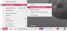
If you select the Similar sub menu when in vertex edit mode Blender already offers a few options to extend your current selection of vertices.

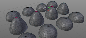
And although useful I frequently find myself in a situation where the available options are not sufficient. Especially in hard edge modeling of objects with identical sub parts I often want to be able to select vertices that not just share the same number of faces but where the these shared faces have something else in common. For example in the object shown below we have two different collections of bumps but the is no way to select just all the spiky tips in one go.

The simple add-on I present here fills this gap: it checks not only if vertices have the same number of surrounding faces but also whether the average angle between the face normals and the vertex normals is similar. This will allow you to distinguish between flat and spiky. The amount of similarity can be tweaked to allow for round-off errors or non smooth meshes.

Availability and usage

After downloading, installing and enabling the add-on from GitHub, the new selection option is available in vertex edit mode from the Select -> Select_similar -> Neighborhood

Black Friday - Cyber Monday at Blender Market

Goods news for cost conscious Blenderheads: from november 25th - november 28th Blender Market will host the yearly Black Friday - Cyber Monday sale!


I will participate will all my products, including my new IDMapper add-on. So if you want to save 25% on WeightLifter, SpaceTree, IDMapper (video) or one of my books, head over to my shop on Blender Market this weekend. Of course many other creators will be participating as well so you might want to shop around a bit more :-)

[For Europeans: remember Blender Market runs on Chicago time, so don't start shopping too early next Friday :-) ]

IDMapper - a complete walkthrough

uploaded a complete walkthrough video to showcase the use of IDMapper.
IDMapper is available on Blender Market.

IDMapper - create ID-maps the easy way

it's always exiting to announce a new product on Blender Market and today I am pleased to announce IDMapper.


IDMapper is a Blender add-on that lets you create a vertex color layer that can be used as an ID-map by texture paint tools like Substance Painter.

When creating textures for models you often want to reduce the actual number of textures, for example because your GPU can only handle a limited number of textures or maybe simply because juggling a large number of textures for a single model is such a hassle.

Whatever your motivation, texture painting software lets you apply different materials to a texture with ease but you still need to identify areas. An ID-map makes it very simple to apply a material to faces that have a certain color, often by letting you pick a color from the ID-map with an eye-dropper tool.

You will still need to create the vertex color layer that can be used as an ID-map and that's where IDMapper can help.

The first thing it offers are powerful heuristics to assign a unique vertex color to regions consisting of related faces. What is considered related can be tweaked interactively and any resulting distinct regions with very similar geometry can still be assign the same vertex color, simplifying for example the assignment of colors in hard-ops modelling in situations where your mesh contains repeated features like handles or bolts.

The second feature is an operator that acts like a new face paint mode. Instead of applying blended colors to vertices in a painterly manner as with Blender's vertex paint mode, this operator keeps colors uniform across a face, something often desirable when assign materials to mesh parts. It also lets you assign new colors to colored regions and resize or smooth these regions interactively.

And finally it offers some convenience functions to combine different vertex color layers and copy vertex color layers from one mesh to another, probably more high poly, mesh.

A short video showcasing the main features is available on Youtube:


IDMapper is available in my Blender Market shop

Blender conference discount at Blender Market


it's becoming a tradition and it is a good one: many products on Blender Market will carry a discount of 20% during the Blender Conference [28 - 30 October].

Of course I will participate all my products so if your were thinking of getting some nice asset or add-on this might be the perfect time.


NodeSet: tiny update might save even some more time

NodeSet is now also available in a Pro version. Read all about it in this article or check out my BlenderMarket shop if you are interested.

In a previous article I showed a small add-on that lets you import a set of textures with a common base name (like the ones typically exported by Substance Painter). It not only groups them in a frame but also gives the individual textures proper labels and sets the non color data attribute accordingly. On top of that you only have to select one textures from a set and all corresponding textures will be loaded anyway.

This should save you quite a lot of time but I found that in real life a complex model or scene can easily have several tens of texture sets, maybe even a hundred or so and multiplied by 5 textures in a typical PBR Metal Rough export (BaseCOlor, Metallic, Height, Normal and Roughness) this results in hundreds of textures and a very cluttered file selector.

Now becuase you only need to select one of them to load the whole set, I made a small change the set the default filter to *Color* so that the file selector will only show the base color files (which happen to be the most distinct ones when you are looking at thumbnails). This reduces the list of files greatly, making it easier to pick the texture set you need (because as sais, clicking just BaseColor will load the others just the same). You can of course always uncheck the filter icon (at the top of the file selector) if necessary.

Code availability

The update is available from GitHub

Check the previous article for info on how to use the add-on. It includes a small tutorial video.

NodeSet: import Substance Painter textures into Blender

NodeSet is now also available in a Pro version. Read all about it in this article or check out my BlenderMarket shop if you are interested.

I recently bought Substance Painter because i really liked the product. But when i started working in ernest on a complex model with a large number of materials, the repetative work necessary to import the relevant textures quickly got tedious.

Of course with Node Wrangler you can import multiple textures at a time but i still had to switch most textures to non color data and the labels on the image texture nodes reflected the filenames which are too long to act as a readable label.

So i decided to create a small add-on that sort of does what Node Wrangler's multiple images does but in a neater way. The add-on is called NodeSet and when you select its menu entry from the node editor (Add->Texture->Set of images) it will:

  • open a file dialog where you can select a texture (you only have to select one from the set of textures)
  • add this texture as an image texture node
  • set the non color data flag if it is not a color texture (i.e. not a BaseColor nor a Diffuse map)
  • automatically try to load all other textures with the same base name (for example Roughness and Metallic). It will ignore textures that are not present
  • give all nodes a descriptive name (BaseColor, Normal, Specular, ...)
  • group all those nodes into a frame with a label that reflects the basename of the texture set
  • order the nodes alphabetically (BaseColor will always be located above Metallic, regardless of the number of textures in the set or the loading order)

The result looks neat and descriptive:


A small tutorial on how to use it is available as well:

This all works because textures exported by Substance Painter normally follow a strict naming convention where each texture in a set has the same basename (typically the meshname followed by the material name) and a different suffix depending on the type of texture (_Normal or _BaseColor for example)

You can change these suffixes when you export so although NodeSet is configured with the Substance Painter defaults for both the metal/roughness and glossiness workflows (i.e. in Substance Painter you can select Export Textures en select either PBR MetalRough or SpecGloss (non PBR)), you can configure the suffixes it will look for in the User preferences -> Addons . If you leave one empty it will not try to load it. There is of course nothing Substance Painter specific in this setup so it should work for every program that is able the produce texture sets with a common basename and a different suffix for each map.

Currently it will look for png, jpg/jpeg, hdr and exr textures.

Availability

The add-on is available from GitHub. Download it and then select it from File -> User preferences -> Add-ons -> install from file. Don't forget to check the enable checkbox.

Creating Add-ons for Blender on Blender Market

Hurray! Now my latest book on creating add-ons for Blender is also available on Blender Market:


(click on the image to go to the shop where you can read the description and download a sample chapter)

To celebrate this event I marked down the price significantly for all the products in my Blender market shop, both e-books and add-ons, so you might want to grab your chance while it lasts!

Open Shading Language for Blender on BlenderMarket

The last couple of weeks I have been working to create a distribution channel for my Blender related e-books that is better suited to the intended audience. And what better distribution channel than BlenderMarket! With special thanks to Jonathan and Matthew I am happy to announce the first result is there:
Open Shading Language for Blender is now also available on BlenderMarket:

(click on the image to go to the shop where you can read the description and download a sample chapter)

A Bugatti T59 modeled in Blender

I normally focus my Blender activities on writing add-ons but I am pretty pleased with this small project:

New Book: Creating add-ons for Blender

Yeah, it's there! I am happy to announce my new, short-and-sweet, information packed book on creating add-ons for Blender.

It might be small, but it is beautifully formed :-) You might want to sample it (or buy of course) from the location below:

A sample of the book is also available as pdf

Small fix to basket arch add-on

Something in the 2.77 Blender API of object_utils.py was changed and broke the basket arch add-on. I fixed it and a new version is available on GitHub.

troubles, troubles, troubles ...

I forgot to renew the lease on the swineworld.org domain with NetworkSolutions. This sucks big time because I cannot remember/ find my login credentials and apparently I never updated my primary email address :-( Asking a question requires that you login and the telephone number listed for international users connects but is not answered!

Well too bad. The old blenderthings.blogspot.com keeps on working but unfortunately all links pointing to www.swineworld.org are now broken, even the ones inside articles that link to other articles on the same blog. I'll try and fiz that as much as I can but I am certainly not renewing this domain with Network Solutions because the first thing they did is auctioning it of for a ridiculous price.

Floor boards add-on: random thickness

Acting on a question from Ákos I added a random thickness option to the add-on.

The new version is of course available on GitHub. (this is a single python file: select File->Save As... from your browser and save it somewhere as planks.py. Then in Blender, select File->User preferences->Add-ons->install from file... (don't forget to remove an earlier version if you have one).

If you select a non-zero thinkness each plank gets a random extra thickness up to the chosen maximum.

The option is located together with the other randomization options (which can be applied in parallel.)

Weightlifter Watershed Demo

I just uploaded a new version of my WeightLifter add-on to BlenderMarket.

The video gives a short impression of the new watershed mode. You could use this watershed mode for example to calculate a realistic distribution of vegetation in large scale landscapes.

Performance of ray casting in Blender Python

The Python API for ray casts on objects and scenes was changed in a breaking manner in Blender 2.77. And because several of my add-ons depend on it, I not only had to fix them but I decided to have a look at the performance as well.
The central use case for ray casting in these add-ons is to check whether a point lies inside a mesh. This is determined by casting a ray and checking if the number of intersections is even or odd (where we count 0 as even). An even number of crossings means the point lies outside the mesh (true for the red points in the illustration) while an odd number means that the point lies inside the mesh (the green point). And the fun part is that this is true for any direction of the ray!

Code

We can easily convert this to Python using Blenders API: given an object and point to test, we take some direction for our ray (here right along the x-direction) and check if there is an intersection. If so, we we test again but start at the intersection point, taking care to move a tiny bit along the ray cast direction to avoid getting 'stuck' at the intersection point due to numerical imprecision. We count the number of intersections and return True if this number is odd.

 
import bpy
from mathutils import Vector
from mathutils.bvhtree import BVHTree

def q_inside(ob, point_in_object_space):
 direction = Vector((1,0,0))
 epsilon = direction * 1e-6
 count = 0
 result, point_in_object_space, normal, index = ob.ray_cast(point_in_object_space, direction)
 while result:
  count += 1
  result, point_in_object_space, normal, index = ob.ray_cast(point_in_object_space + epsilon, direction)
 return (count % 2) == 1

Intersection with an object

We can now use this function to determine if a point lies within a mesh object:
        q_inside(ob, (0,0,0))
Note that the point to check is in object space so if you want to check if a point in world space lies within the mesh you should convert it first using the inverted wordl matrix of the object.

Intersection with a precalculated BVH tree

To determine if a ray hits any of the possibly millions of polygons that make up a mesh, the ray_cast() method internally constructs something called a BVH tree. This is a rather costly operation but fortunately a BVH tree is cached so when we perform many intersection tests this overhead should pay off. BVH trees however can also be constructed from a mesh object separately and offers exactly the same signature ray_cast() method. This means we can perform the same check to see if a point lies inside a mesh with following code:
    sc = bpy.context.scene

    bvhtree = BVHTree.FromObject(ob, sc)

    q_inside(bvhtree, (0,0,0))

Performance

When doing millions of tests on the same mesh a small amount of overhead averages out so the question is if it is meaningful to create a separate BVH tree. If we look at the time it takes to do a million tests for meshes of different sizes we see that the overhead apparently is not the same but for larger meshes this difference loses significance:

inside irregular mesh (subdivided Suzanne)

facesobjectbvhtreegain%
1280003.5473.2418.6
320003.5261.89246.3
80003.4731.71550.6
20003.3931.63951.7
5003.3911.59752.9

outside irregular mesh with mostly immediate initial hit

The initial data was for a point inside a mesh: such a point will always need at least two ray casts: the first will intersect some polygon, the second will veer off into infinity. If we test a point outside a mesh we sometimes will have only one ray cast and sometimes two. if we look at the latter scenario we see similar behavior:
facesobjectbvhtreegain%
1280003.6083.14812.7
320003.4341.83646.5
80003.3811.63751.6
20003.2771.55852.4
5003.2941.52853.6

outside irregular mesh with mostly no initial hits

A strange thing happens when the point to test is outside the mesh but the ray happens to point away from the mesh so that we will have zero intersections. Now for large meshes the overhead of a separate BVH tree appears larger!
facesobjectbvhtreegain%
1280001.5342.417-57.6
320001.5441.01134.5
80001.520.83245.2
20001.5230.79647.7
5001.5340.78349

Conclusion

i cannot quite explain the behavior of the ray_cast() performance for larger meshes when the point is outside the mesh and the test ray points away, but in arbitrary situations and moderately sized meshes a perfomance gain of 40% for the BVH tree is worthwhile when doing millions of tests.

Floor boards add-on: another small feature

Again prompted by a question I added a feature to guarantee minimum plank lengths at the sides when using random plank lengths, to mimic real life behavior where you would not allow too short ends when laying a wooden floor.

In practice you would probably also try to avoid seams to line up in adjacent rows but if this happens you can easily switch to another random seed already.

The images below show the vertex color map (for clarity) with (left) and without a minimum offset of 12 cm, resulting in less short 'stubs'.

Availability

As usual the latest version is available on GitHub.

Other floor board articles

This blog already sports quite a number of articles on this add-on. The easiest way to see them all is to select the floor board tag (on the right, or click the link).

Calculating the number of connections in a tree, or why numpy is awesome but a good algorithm even more so

the issue

imagine you are creating trees, either pure data structures or ones that try to mimic real trees, and that you are interested in the number of connected branch segments. How would you calculate these numbers for each node in the tree?
If we have a small tree like the one in the illustration, where we have placed the node index inside each sphere, we might store for each node the index of its parent, like in the list: p = [ -1, 0, 1, 2, 2, 4 ]Note that node number 0 has -1 as the index of its parent to indicate it has no parent because it is the root node. Also node 3 and 4 have the same parent node because they represent a fork in a branch.

naive solution

to calculate the number of connected nodes for each node in the tree we could simply iterate over all the nodes and traverse the list of parent nodes until we reach the root node, all the while adding 1 to the number of connections. This might look like this (the numbers are profiling information)
      hits       time      t/hit

      7385       4037      0.5   for p in parents:
    683441    1627791      2.4    while p >= 0:
    676057     410569      0.6     connections[p] += 1
    676057     351262      0.5     p = parents[p]
The result has the following values c = [5, 4, 3, 0, 1, 0]The tips have no connections while the root counts all nodes as connections minus itself so our 6-node tree had a root with 5 connections. This is also illustrated in the illustration (on the right).
If we time this simple algorithm for a moderately sized tree of just over 7000 nodes (which might look like the one in the image below to get a sense of the complexity) I find that it takes about 1.16 seconds on my machine.

numpy implementation

Now we all know that numpy is good at working with large arrays of numbers (and conveniently already bundled with Blender) so we might try some simple changes. Almost identical code but with numpy arrays instead of python lists:
      hits       time      t/hit

      7385       4563     0.6   for p in self.parent[:self.nverts]:
    683441    1695443     2.5    while p >= 0:
    676057    2004637     3.0     self.connections[p] += 1
    676057     456995     0.7     p = self.parent[p] 
But in fact this is slower! ( 2.68 seconds on my machine) If we look at the timings from the excellent kernprof line profiler (the numbers on the left of the code snippets) we see that numpy spends an awful lot of time on both the iteration over the parents and especially the indexing of the connection array. Apparently indexing a single element in a numpy array is slower than the equivalent operation on a python list. (There is a good explanation why indexing a single element of a numpy array takes so long on StackOverflow.)

reworking the algorithm

It must be possible to do this faster right? Yes it is, have a look at the following code:
      hits       time      t/hit

         1           2      2.0   p = self.parent[:self.nverts]
         1          19     19.0   p = p[p>=0]
       137          97      0.7   while len(p):
       136        1684     12.4    c = np.bincount(p)
       136        1013      7.4    self.connections[:len(c)] += c
       136        3395     25.0    p = self.parent[p]
       136        1547     11.4    p = p[p>=0]
This produces the same result (trust me, i'll explain in a minute), yet uses only milliseconds (7 to be precise). The trick is to use as much numpy code with looping and indexing built in as possible: bincount() counts the number of occurrences of a number and stores it the corresponding bin. So if 3 nodes have node 0 as their parent, c[0] will be 3. Next we add this list in one go to the cumulative number of connections and finally we get the parent indices also in a single statement and remove the -1 entries (those nodes that reached root in their tree traversal). We repeat this as long as there are nodes that have not yet reached root.

conclusion

Numpy might often be faster than pure Python but it pays to check, using careful profiling. Using an appropriate algorithm that does away as much as possible with any python overhead might however give you a sizeable speed improvement although the algorithm might not be immediately obvious to find.

Space tree pro

This bit of research is not just academical, I am currently investigating options to speed up tree generation as implemented in my Space Tree Pro Blender add-on (available on BlenderMarket)


Floor boards add-on: minor feature added

Prompted by a question from Trevor I added a Restricted random mode to the uv randomization. It still randomizes the position of planks on the uv-map but keeps them inside the original bounds. It does this simply by not moving a uv map of a plank at all when the move would result in any portion of the plank ending up outside the bounds. The result is a compacter randomized uv-map which should make it somewhat easier to use with non-tiling textures, i.e. reduce the area of the textures that is not used.

The new version is of course available on GitHub.

The difference is illustrated in the image below where I have contrasted the random uv-map in orange with the restricted uv-map in green

random vertex colors using Numpy

The bit of research presented in a previous article was not completely academical: speed improvements using Numpy are very welcome when for example generating random vertex colors for very large meshes.
With the results of the measurements in the back of my mind and spurred by a discussion on BlenderArtists I created a new version of the random vertex colors addon. (available on GitHub), which reduced the time to generate random vertex colors for approximately 1 million faces from 3.2 seconds to 0.8 seconds on my machine (or even 0.4s for a 32 bit variant), i.e. up to 8 times faster which is not bad.

Some explanation

Assigning random vertex colors to faces means that you have to assign colors to all the loops of a polygon the same random color (for the difference between vertices and loops, check the BMesh design document. The same applies to the regular Mesh objects we use in the code below). This can be done in a straight forward manner once you have located the vertex color layer:
mesh = context.scene.objects.active.data
vertex_colors = mesh.vertex_colors.active.data
polygons = mesh.polygons
for poly in polygons:
 color = [random(), random(), random()]
 for loop_index in range(poly.loop_start, poly.loop_start + poly.loop_total):
  vertex_colors[loop_index].color = color
Straight forward as this may be, a loop inside a loop is time consuming and so is generating lots of random numbers, especially because Python does not do this in parallel even if you have a processor with multiple cores. Fortunately for us Blender comes bundled with Numpy, which is a library that can manipulate huge arrays of numbers in a very efficient manner. This allows for a much more efficient approach (although as shown previously a significant speed increase is only noticeable for large meshes).
startloop = np.empty(npolygons, dtype=np.int)
numloops = np.empty(npolygons, dtype=np.int)
polygon_indices = np.empty(npolygons, dtype=np.int)

polygons.foreach_get('index', polygon_indices)
polygons.foreach_get('loop_start', startloop)
polygons.foreach_get('loop_total', numloops)

colors = np.random.random_sample((npolygons,3))
We can even reduce storage (and get an additional speedup) if we change the types to 32 bit variants. There will be no loss of accuracy as these are the sizes used by Blender internally. (Would you do a lot of additional calculations this might be different of course). The change would only alter the declarations of the arrays:
startloop = np.empty(npolygons, dtype=np.int32)
numloops = np.empty(npolygons, dtype=np.int32)
polygon_indices = np.empty(npolygons, dtype=np.int32)

polygons.foreach_get('index', polygon_indices)
polygons.foreach_get('loop_start', startloop)
polygons.foreach_get('loop_total', numloops)

colors = np.random.random_sample((npolygons,3)).astype(np.float32)
As shown above we start out by creating Numpy array that will hold the startloop indices and the number of of loops in each polygon as well as an array that will hold the polygon indices itself. This last one isn't strictly needed for assigning random values because we don't care which random color we assign to which polygon but for other scenarios it might make more sense so we keep it here. We get all these indices from the Mesh object using the fast foreach_get method. We then use Numpy buil-in random_sample function the generate the random colors (3 random floats between 0 and 1) for all polygons.
loopcolors = np.empty((nloops,3)) # or loopcolors = np.empty((nloops,3), dtype=np.float32)
loopcolors[startloop] = colors[polygon_indices]
numloops -= 1
nz = np.flatnonzero(numloops)
while len(nz):
 startloop[nz] += 1
 loopcolors[startloop[nz]] = colors[polygon_indices[nz]]
 numloops[nz] -= 1
 nz = np.flatnonzero(numloops)
The real work is done in the code above: we first create an empty array to hold the colors for all individual loops. Then we assign all the loops with index startloop with the colors that corresponds to the color of the polygon it belongs to. Note that startloop and polygon_indices are arrays with the same length, i.e. the number of polygons. Now we also have an array numloops which holds for each polygon the number of loops. We decrement this number of loops by one for all polygons in one go (line 3) and create an array of indices of those elements in numloops that are still greater than zero (line 4). If we are still left with one or more indices (line 5) we increment the index of the startloop for all those nonzero indices (line 6).
Line 7 then assigns again in one go a polygon color to a loop at a certain index for all polygons where there are still a non zero number of loops. And finally we again reduce our numloop counters. Note that this all works because the loop indices of all loops of a polygon are consecutive.
loopcolors = loopcolors.flatten()
vertex_colors.foreach_set("color", loopcolors)
The final lines flatten the array of loop colors to a 1-D array and write back the colors to the Mesh object with the fast foreach_set method.

Discussion

Now even though we end up with about four times as much code, it is much faster while still quite readable, as long as you get your head around using index arrays. Basically our single while loops executes the inner loop of assigning colors to loops for all polygons in parallel. The penalty is for this speed increase is memory consumption: We use 5 large numpy arrays here.

Copying vertices to Numpy arrays in Blender

If you want to do a lot of mathematical work on very large Blender meshes using plain Python might be too slow. Fortunately Blender comes bundled with Numpy which allows for fast calculations on vast arrays of numerical data.
To use Numpy you would need to copy for example vertex coordinates first before performing any calculations and then copy the results back again. This consumes extra memory and time. You wouldn't do this for a single operation like determining the average position of all vertices because Python can perform this so efficiently that it wouldn't compensate the extra setup time. However, when calculating many iterations of some erosion algorithm this might be well worth the cost.
In order to help in deciding whether this setup cost is worth the effort I decided to produce some benchmark values. My aim was to find the fastest method from several alternatives and to produce actual timings. Now your timings will be different of course but the trends will be comparable and I have provided the source code for my benchmark programs on GitHub.

results, copying to a Numpy array

First we have a look at how much time it takes to copy the vertex coordinates from a mesh to a Numpy array. Given a the array of vertices me.vertices and a Numpy array verts we have several options:
# blue line
verts = np.array([v.co for v in me.vertices])

# red line
verts = np.fromiter((x for v in me.vertices for x in v.co),
                     dtype=np.float64)
verts.shape = (len(me.vertices), 3)

# orange line
verts = np.fromiter((x for v in me.vertices for x in v.co),
                     dtype=np.float64,
                     count=len(me.vertices)*3)
verts.shape = (len(me.vertices), 3)

# green line
verts = np.empty(count*3, dtype=np.float64)
me.vertices.foreach_get('co', verts)
verts.shape = shape
The blue line represents the creating of a Numpy array from a list. Even with list comprehension this has the disadvantage of creating a intermediate copy, which is also a Python list. Apparently this a costly operation as this naive method performes the worst of all.
The red line shows a huge increase in performance as we use a generator expression to access the coordinates. This will not create an intermediate list but the result is a one dimensional array. Changing the shape of an array in Numpy involves no copying so is very cheap.
We can still improve a little bit on our timing by preallocating the size for the Numpy array. The result is shown with the orange line.
The green line shows the fastest option. Blender provides a fast method to access attributes in a property collection and this method wins hands down. (thanks Linus Yng for pointing this out)

results, copying from a Numpy array

Copying data back from a Numpy array can also be done in more than one way, the most interesting ones are shown below:
# blue line
for i,v in enumerate(me.vertices):
    v.co = verts[i]

# green line
for n,v in zip(verts, me.vertices):
    v.co = n

# light blue line
def f2(n,v):
    v.co = n

for v in itertools.starmap(f2, zip(verts, me.vertices)): pass

# orange line
verts.shape = count*3
me.vertices.foreach_set('co', verts)
verts.shape = shape
The conventional methods perform not significantly different, but again Blenders built-in foreach_set method outperforms all other other options by a mile, just like its foreach_get counterpart.


Discussion

The actual timings on my machine (a intel core i7 running at 4GHz) indicate that we can copy about 1.87 Million vertex coordinates per second from a Blender mesh to a Numpy array and about 1.12 Million vertex coordinates per second from a Numpy array to a Blender mesh using 'conventional methods'. The 50% difference might be due to the fact that the coordinate data in a Blender mesh is scattered over the internal memory (as compared to Numpy's contiguous block of ram) and writing to scattered memory incurs a bigger hit form cache misses and the like than reading from it. Note that a vertex location consists of three 64 bit floating point numbers.
Using foreach_get and foreach_set this performance is greatly improved to 13.8 Million vertex coordinates per second and 10.8 Million vertex coordinates per second respectively (on my machine).
Overall, with this performance this means that on my machine even a simple scaling operation on a million vertices might already be faster with Numpy, like shown in the first example below, which on my machine is about 7x faster (not that scaling is such a perfect example, chances are Blender's scale operator is faster but it gives you an idea how much there is to gain if even for simple operations that are not natively available in Blender.
    # numpy code with fast Blender foreach
    fac = np.array([1.1, 1.1, 1.1])
    count = len(me.vertices)
    shape = (count, 3)
    
    fac = np.array([1.1, 1.1, 1.1])

    verts = np.empty(count*3, dtype=np.float64)
    me.vertices.foreach_get('co', verts)
    verts.shape = shape
    np.multiply(verts,fac,out=verts)
    verts.shape = count*3
    me.vertices.foreach_set('co', verts)
    verts.shape = shape

    # 'classic code'
    fac = Vector((1.1, 1.1, 1.1))

    for v in me.vertices:
        v.co[0] *= fac[0]
        v.co[1] *= fac[1]
        v.co[2] *= fac[2]

Benchmark availability

The .blend file with code and instructions can be downloaded from my GitHub repository.


Blender add-on: create a camera view filling backdrop

whether for product presentations or outdoor scenes, often you need a backdrop that nicely fills the camera view, preferably with a nice curve upwards to hide the horizon and also not larger than necessary to reduce the number of vertices and particles.

Creating this by hand is not massively time consuming but tedious enough to benefit from a small add-on: BackDrop.

Features

By default it creates a flat horizontal mesh at z=0 that fills the camera view exactly. By working with the margin option you can create a backdrop that is slightly bigger than the exact view and unchecking the Zero level option will allow you to position the backdrop on another z-coordinate.

The Lift option will elevate the far end of the backdrop resulting in a curved mesh. The curvature can be adjusted but that doesn't work well yet.

The backdrop mesh is parented to the camera so it will move with it if you rotate or translate the camera.

Availability

The plugin is available on my blenderaddons project on GitHub. Just download backdrop.py and install it from File -> user preferences -> Add-ons -> install from file

Bugs and limitations

The plugin cannot in all circumstances create a suitable backdrop, for example if the camera is pointing upward. If this is the case, a suitable error is displayed in the properties in the toolbar.

Also, the curvature control sucks, and in fact create a curves surface using bezier interpolation is not optiomal since the points are not evenly spaced. For this we need to convert it to an arc length parameterization but I don't have time to do that now.

DumpMesh: clean, complete, sexy

The previous bugfix release of DumpMesh was already able to dump quite a number attributes and attribute layers but in the latest version I went the whole way and dumped every attribute layer that happens to be defined. And I really mean every layer: if you have added a skin modifier the BMSkinVert layer will be dumped for example and even if you assign values to the generic float, string, etc. attribute layers programmatically the will be dumped as well.

Note that vertex groups will not be dumped: vertex groups are not part of a mesh but of an object. (yes, if you didn't know that already, you can have more than one object pointing to the same mesh data, each with its own vertex groups)

This is done by code that is a lot more Pythonic (whatever that means, for me pragmatism is more important than style, as long as it is readable and documented). It uses a lot of introspection to keep the code short and sweet as well. Of course it helps that Blender attribute layers (aka CustomData) is very flexible and well designed (well,... mostly, see Bugs below)

Functionally the add-on hasn't changed much: the interface is cleaner (no more separate selection of what will be dumped, you either choose just geometry or everything), and now all objects that are selected are dumped. This might give a slightly faster workflow.

Availability

The updated code for DumpMesh and CreateMesh can be found on my GitHub repository. DumpMesh can be downloaded directly from this link, as can CreateMesh if your are interested to look at the code.

Bugs

Blenders Python API is generally well designed and adequately documented but there are still some bugs and strange design issues:
BMVertSkin
not documented at all but it is used by the skin modifier. And the bm.verts.layers.skin layer the skin modifier creates has a name that is an empty string
BMTexPoly
has a documentation entry but is marked as todo. Fair enough, because this might be for Ptex stuff that is sort of shelved for now. In the add-on it is mostly ignored.
bm.loops.index_update()
If you add vertices, edges or faces to a bmesh you must ensure that the sequences they are members of can be indexed. You can do this with bm.verts.ensure_lookup_table() or equivalent. If you not only need to be able to do bm.verts[i] but need the actual index as well, like bm.verts[i].index you need to call bm.verts.index_update() otherwise all indices are -1. So far so good, however for loops this appears to be either unfinished or I don't understand it: there is no ensure_lookup_table() for loops, apparently this is taken care of by the faces, but any index attribute of a BMLoop is -1. now bm.faces[i].loops does have an index_update() but it will generate only indices for the loops of that particular face and will start at 0. However when transfering a bmesh to a regular mesh the indices of all loops in the whole mesh are properly initialized, so there is apparently hidden functionality to take care of this. Of course most of the time you can do without but in the addon I dump loop layers as dictionaries of dictionaries that can be indexed as d[faceindex][loopindex] where loopindex is initialy derived from the complete mesh and therefore numbered as one unbroken sequence of all the loops.
factories instead of instantiation from a class
BMesh, BMVert, BMSinVert, etc. are not fully fledged classes. You cannot subclass them and you cannot instantiate them with BMesh(). also most have no __repr__() function and also cannot be pickled. This means that especially for layer attributes like BMSkinVert with more than one attribute you have to know what to assign to which attribute, which is cumbersome. introspection is no help here because you cannot know which attribute is to be saved and which one is just for temporary use.
These aren't deal breakers, just things to keep in mind when you are designing an add-on.

Blender add-on: DumpMesh [Update]

In a previous article I presented a small add-on that could dump all sorts of mesh characteristics like vertex coordinates, faces, edges, seams, etc. as Python code. This code could then be included in other add-ons for example to be used as basic building blocks for parameterized objects.
I have now added the edge selection status and the active uv-map to the list of items that can be dumped. I also fixed a couple of bugs and made dumping most characteristics optional. DumpMesh not only dumps mesh information into a text block but optionally also generates complete add-on code to regenerate the mesh. It serves both as a way to test the generated Python data and might serve as an example of how to create a bmesh object from scratch, including how to add data layers for edges (crease) and loops (uvs).
From a Python point of view DumpMesh.py might be interesting because I had to find a way to include a large chunk of Python code as a string (the source code for the CreateMesh add-on). I solved this by including this source code as a base64 encoded string that is decoded on the fly. This way any quotes or other nasty stuff won't cause the same challenge as trying to create a string literal (which would contain quotes but also escaped quotes etc...).
CreateMesh was even more challenging in a way: DumpMesh generates source code that defines all sorts of list. However, many of these list are optional and all might have a suffix chosen by the user. This means that the CreateMesh add-on must have a way to check if the lists are defined. Fortunately this information is readily accessible in Python because any globally defined variabele is an entry in the dict returned by globals(). Anyway, some annotations can be found at the end of this article.

Availability

The updated code for DumpMesh and CreateMesh can be found on my GitHub repository. DumpMesh can be downloaded directly from this link, as can CreateMesh if your are interested to look at the code.

CreateMesh Python tricks

The lists and dicts with data created by DumpMesh look like this:
suffix = ""

verts = [(-1,-1,-1),(-1.0365,-1,1.0122), ... ]

faces = [(1, 3, 2, 0),(3, 7, 6, 2), ... ]

edges = [(0, 1),(1, 3),(3, 2),(2, 0), ... ]

seams = {0: False,1: False,2: False,3: ... }

crease = {0: 0.0,1: 0.0,2: 0.0,3: 0.0,4: ... }

selected = {0: True,1: True,2: True,3: ... }

uv = {0: {1: (0,0),3: (1,0),2: (1,1),0: (0,1),}, 1: ... }
With a suffix the code would look something like this:
suffix = "_cube"

verts_cube = [(-1,-1,-1),(-1.0365,-1,1.0122), ... ]

faces_cube = [(1, 3, 2, 0),(3, 7, 6, 2), ... ]

edges_cube = [(0, 1),(1, 3),(3, 2),(2, 0), ... ]

...
The geometry() function that creates a bmesh from this data has be clever because for example seams might not be defined at all or might not be called seams but seams_cube for example. This is solved by checking the dict of global symbols returned by globals():
def geometry():

 # we check if certain lists and dicts are defined
 have_seams  = 'seams' + suffix in globals()
 have_crease  = 'crease' + suffix in globals()
 have_selected  = 'selected' + suffix in globals()
 have_uv  = 'uv' + suffix in globals()

 # we deliberately shadow the global entries so we don't have to deal
 # with the suffix if it's there
 verts = globals()['verts' + suffix]
 edges = globals()['edges' + suffix]
 faces = globals()['faces' + suffix]
 if have_seams: seams = globals()['seams' + suffix]
 if have_crease: crease = globals()['crease' + suffix]
 if have_selected: selected = globals()['selected' + suffix]
 if have_uv: uv = globals()['uv' + suffix]

BMesh pitfalls

A peculiarity of the way BMesh works is that adding elements like verts or edges to their respective lists does not guarantee that they are indexable! That means that after adding a number of vertices you must call bm.verts.ensure_lookup_table() in order to access a vertex as for example bm.verts[3]. Now they rela tricky part is that being able to index the list of verts is not sufficient to get the index of a vertex! That is, if you want to retrieve bm.verts[3].index you need to call bm.verts.index_update() first. Even though this is documented here and here, it baffled me at first. (note: what goes for verts, goes for edges and faces as well). So for verts the complete code looks like this:
 bm = bmesh.new()

 for v in verts:
  bm.verts.new(v)
        # ensure bm.verts can be indexed
 bm.verts.ensure_lookup_table()
        # ensures all bm.verts have an index (= different thing!)
 bm.verts.index_update()


Blender add-on: DumpMesh

DumpMesh is an add-on that will write a lot of information about a currently selected mesh object in the form of Python code. The resulting code is stored as a text object in the Text Editor.
Of course it is far more effective to store an object by saving the .blend file and reuse it afterward but the purpose of this add-on is to get access to mesh data in a form that can easily be used in other add-ons, for example as the basis of some parameterized object, where creating lists of vertex coordinates by hand is very tedious and error prone. It therefore produces Python definitions for
  • a list of vertex coordinates
  • a list of edges
  • a list of faces
  • a dictionary with edge seams
  • a dictionary with edge creases
A small, shortened, example of what is produced is shown below:
verts = [
 (-1.0, -1.0, -1.0),
 (-1.0, -1.0, 1.0),
...
 (1.0, 1.0, 1.0),
]

faces = [
 (1, 3, 2, 0),
 (3, 7, 6, 2),
...
 (5, 7, 3, 1),
]

edges = [
 (0, 1),
 (1, 3),
...
 (0, 4),
]

seams = {
 0: True,
 1: True,
...
 11: False,
}

crease = {
 0: 0.0,
 1: 1.0,
...    
 11: 0.0,
}
By default it also produces code for an operator that recreates a mesh object based on the values in the lists and dictionaries mentioned above.
The latter may sound a bit strange, an add-on that produces code for an add-on, but this way it is very simple to verify that the dumped data indeed produces the desired object when used. Your work flow may look like this:
  • Select the object to dump in the 3D view,
  • Select Object -> DumpMesh, the code will show up in the text editor,
  • Run the script in the text editor by clicking Run script, it will create a new menu entry
  • Select Add -> Mesh -> CreateMesh, and a duplicate mesh should be added to your scene.
If satisfied with the result you can save the generated code for reuse in your own add-on.

Availability

The code for DumpMesh is available on GitHub. Just download the file and use File -> User preferences -> Add-ons -> Install from file in the usual manner. In the code I have embedded the code for the CreateMesh operator as base64 encoded strings. This is in my opinion the simplest way to store a chunk of Python in antother Python program without bothering about quotes of all kinds. The original non-encoded version is on GitHub as well.

Noise experiment with Open Shading Language

I am still looking for good procedural noise to be used as the basis for bark materials. Such noise would need some anisotropy because the cracks in bark are almast always oriented: either along the direction of the trunk or perpendicular to it, depending on the stretching characteristics during growth. Now you could scale for example Perlin noise or use Gabor noise (the latter is available in OSL as well, check for example this article), but we could also create it from scratch.

Theory

In the shader we randomly distribute a number of line segments through space and calculate the distance to these line segments. If we are close enough to a segment we add a value to our sum and in the end the value for a pixel is the sum of all these contributions. Now the essence is in the distribution of those line segments because we do not only control their length but also how far they may deviate from a preferred direction.
The code for the shader itself is quite simple (I have omitted all auxiliary functions):
shader dtnoise(
 point  Pos = P,            // texture position and scale
 float  Scale = 1,
 
 int    Np = 15,            // number of ticks (impulse) per cell
 
 int    Seed = 42,          // random seed
 
 float  Radius = 0.3,       // distance to impulse that will add to result
 float  Size = 0.7,         // length of an impulse
 vector Dir = vector(1,0,0),// direction of anisotropy
 float  Theta = M_PI/2,     // cone (half)angle. The default = 90% which means no anisotropy
 
 float  Step = 0.3,         // cutoff value for Fac output
 float  Gain = 0.3,         // brightness of the result
 
 output float Sum = 0,      // the sum of all the tick values
 output float Fac = 0       // the 
){
 point p = Pos * Scale;
 point f = floor(p);

 vector an= normalize(Dir);
 vector r = vector(an[2],an[1],an[0]); //no need to norm again
 vector uv = cross(an,r);
 vector vv = cross(an,u);

 
 int xx,yy,zz, np;
 
 int nn[3];
 
 for( xx=-1; xx<=1; xx++){
  for( yy=-1; yy<=1; yy++){
   for( zz=-1; zz<=1; zz++){
    point ff = f + vector(xx,yy,zz);
    int s=Seed;
    
    nn[0] = int(ff[0]);
    nn[1] = int(ff[1]);
    nn[2] = int(ff[2]);
    
    for( np=0; np < Np; np++){
     vector pd1 = noise("cell",ff,s);
     vector pd2 = randomcone(uv, vv, an, Theta, nn, s+1);
    
     point p1 = ff + pd1;
     point p2 = p1 + Size * pd2;
    
     float d = distance(p1,p2,p);     
     Sum += (1 - smoothstep(0, Radius, d));
     
     s+=3;
    }
   }
  }
 }
 
 Sum *= Gain;
 Fac = smoothstep(0, Step, Sum);
}
The essence is in line 44 and 45: here we pick a random point and another point along a random direction, where this random direction is restricted to a cone whose narrowness we can control with the Theta parameter. Those two points make up the start and end points of a line segment and if the distance to this line segment is small enough we a a value. (make sure that the sum of Size and Length < 1 to prevent artifacts.

Samples

With few points per cell the anisotropy is very clear (left: Theta = 0.05, right Theta = 1.51 (approx. 90 degrees):
   
 Adding points increases the complexity of the noise (we reduced the gain, the number of points is 40):
 
If we compare our noise to gabor and perlin noise (each thresholded and suitably scaled in a preferred direction) we see that the patterns are similar but each with its own character.

How useful this all is, it up to you of course :-) It is nice to have a different procedural noise in your toolbox but on the other hand, it ties you to OSL (i.e. you can't use it on the GPU) and it is relatively slow.

Code availability

As usual the full code is available on GitHub.

Mmmm, maybe this advertising widget below is a bit over sized. Still, if you would like to learn some more about Open Shading Language for Blender, you might check it out.