Drawing cubic splines in OSL

Some time ago I wrote about a routine to calculate the closest distance to a quadratic bezier spline and recently I reused this routine again in a slightly optimized form to create wiggles.
Being able to calculate the closest distance to a quadratic spline is useful but I really wanted to use cubic splines because they offer more control, allowing for easier ways to create nice shapes.

update: made the code 10% faster by making it 2D only. The GitHub version relects that change but original code can be used by removing a single macro
Warning; long read ahead :-) The first section describes how to use the shader and where to download the code and is pretty short. The second section dives deep into the code and is definitely not an easy read, sorry for that but fortunately there is no need to go that deep if you know what a cubic spline is and just want to use the code.

If you would like to know more about programming OSL you might be interested in my book "Open Shading Language for Blender". More on the availability of this book and a sample can be found on this page.

The shader

The approach to finding the distance to a cubic spline is the same in principle as for a quadratic spline: find all values for t that satify the relation dB(t)/dt . (B(t) - P) = 0, or in English: those values of t whre the tangent to the spline is perpendicular to the vector pointing to the point being shaded (remember that the dot product of two vectors is zero if they are perpendicular).
For a quadratic bezier curve the equation to solve is cubic and is quite simple but for a cubic bezier curve this is a fifth order equation for which there is no analytical solution. And although cubic splines are used everwhere (for example in fonts) a numerical solution for this problem was surprisingly hard to find.
Fortunately after some serious searching the Graphic Gems series of books proved again to be incredible useful, specifically "A Bezier Curve-Based Root-Finder" by Philip J. Schneider.
The original code is in C so it neede quite some work to convert it to OSL. Normally converting C code to OSL is pretty straightforward but this code uses multidimensional arrays and recursion, both unknown to OSL. On the plus side, OSL's native point type and built-in dot() make for a lot less code.

Code availability and node setup

My implementation (with a sample shader in the same file) is available on GitHub. The node setup used to create the heart shape is shown below, it is made of two mirrored splines:

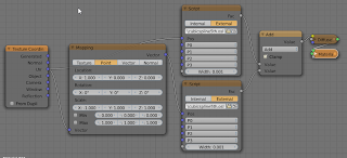
The values for the control points are:P0 = ( 0.5, 0.1, 0.0)
P1 = (-0.5, 0.7, 0.0)
P2 = ( 0.4, 1.2, 0.0)
P3 = ( 0.5, 0.8, 0.0)

Code explanation

I am not going to list all of the code because it's way to long and rather boring but I will tell some more about the FindRoots() which is nontrivial and needed to be reimplemented in a non-recursive form.
The general idea of the shader to cast the fifth order equation whose roots we'd like to find in a form that is itself a bezier curve (I.e. a bernstein polynomial) and exploit the specific properties of a bezier curve to efficiently find the roots.
The mathematical specifics are explained very well in Schneider's article so let us just look at the code:

#define POP wtop+=6;wn--

int FindRoots(point w0[6], float t[5]){
  point w[STACKSIZE];
  int wtop=0;
  int wend=0;
  int wn=0;
  for(int k=0;k<6 br="" k="" w0="" w="" wend="">  wn++;
  int nc=0;
  while(wn>0){
    //printf("[%d]",wn);
    int cc=CrossingCount(w,wtop); // w[:5]
    if(cc==0){
      POP;
      continue;
    }
    if(cc==1){
      if(wn>=MAXDEPTH){
        t[nc++]= (w[wtop][0]+w[wtop+5][0])/2;
        //printf(" MAX ");
        POP;
        continue;
      }
      if(ControlPolygonFlatEnough(w,wtop)){ // w[:5]
        t[nc++]= ComputeXIntercept(w,wtop);
        //printf(" FLAT (%.1f | %.1f)",w[wtop],w[wtop+5]);
        POP;
        continue;
      }
    }
    // not flat or more than one crossing
    DeCasteljau(w,0.5,wtop,wend);  //left=[wend:wend+5], right=[wend+6;wend+11]
    for(int k=0;k<6 br="" k="" w="" wend="" wtop="">    wn++; wend+=6;
  }
  return nc;
}

A fifth order bezier curve has 6 control points and at most 5 roots. The control points are passed as the w0 argument and the t array will receive the root values. The function's return value will be the number of roots found.
The central idea of this algorithm is to find a segment of the curve that crosses the x-axis just once and then determine the intercept, i.e. a root. To achieve this the spline is subdived into to halves, each again a fifth order spline, until such segment contains a single crossing.
Because OSL doesn't support recursion, we have to maintain a stack of control points ourselves and that's where the w array comes in.
Starting with the for-loop in line 8 we transfer the initial set of 6 control points to the stack and adjust wn to reflect that we now have one set on the stack. At this point wtop (the index of the first control point in the topmost set) is 0, and wend (the index of the first free slot in w) is 6. nc holds the number of roots found sofar.
Next we iterate as long as there is a set of control points on the stack (line 11). We caculate how many times the curve defined by this set crosses the x-axis. If there is no crossing there is no root in this curve so we pop the set of the stack and continue.
If there is a single root and we have recursed deep enough we simply approximate the root as lying halfway between the x-coordinates of the first and last control points and pop the set (line 20). If there is room to recurse we check whether the set of control points is "flat enough" (line 25) and if so compute the intercept with the x-axis of the line between the first and last control point. We store this root and pop the set of control points (see Schneider's article or the original source code to see what is meant by "flat enough").
If the control points are not "flat enough" or we have more than one root in this curve, we split the curve in two using DeCasteljau's method (line 33). The function will produce two sets of six control points at position wend in the w array. The save space we copy the second set to top of the stack (because the control points for the original curve are no longer needed), which means we only have to increase the stacksize wn by one.
Finally, if we run out of the while-loop we simply return the number of roots found.

Speed

Now you might think that all this recursion and the numerous calculations would be very slow but you will be surprised. The function seldom needs to recurse very deep because the accuracy used to determine if a curve is "flat enough" need not be that good (we can't see differences much less than a pixel). On my machine this means that I can tweak the node setup for the example image at interactive speeds if I set the number of preview samples to 1.
There is however plenty of room for optimization, especially in areas were we do calculations with 3D points. If we only want to work in 2D we might save up to 30% on unnecessary calculations.

Creating unique snowflakes with OSL

Falling snowflakes are easy enough to dimulate in Blender with a particle system but if quite a few of them might be seen fairly close up, the real challenge is in making sure each one is unique.

The shader presented in this article will create a unique snowflake for each value of its Seed. Using the object info node we may obtain a unique random number for each object that we may use for this purpose as we will see when we examine the node setup.

Snowflakes

The code below defines the following utility functions;

hex

this function will produce the x and y coordinates of a point as it is rotated through the six segments of a hexagon

in_hexagon

this function will return a non zero value if a point lies within a hexagon

pattern

this function does the real work. It returns non zero if a point is positioned within a number of hexagons that are randomly positioned along the x-axis. It also draws a connecting rod that extends as far as the farthest hexagon.

The body of the shader itself just copies the position being shaded along a hexagon and then calls pattern(). Note that because we expect uv-coordinates for a simple square (I.e in de range [0,1], we transform these coordinates so that the center is at (0.5, 0.5) [line 68].

#define SLOPE 1/sqrt(3)
#define SIDE sqrt(.75)
#define D60c cos(radians(60))
#define D60s sin(radians(60))
 
void hex(float x, float y, output float hx[6], output float hy[6]){
  hx[0]=x;
  hy[0]=y;
  hx[1]=x*D60c-y*D60s;
  hy[1]=y*D60c+x*D60s;
  hx[2]=x*D60c+y*D60s;;
  hy[2]=y*D60c-x*D60s;
  hx[3]=-hx[0];
  hy[3]=-hy[0];
  hx[4]=-hx[1];
  hy[4]=-hy[1];
  hx[5]=-hx[2];
  hy[5]=-hy[2];
}

int in_hexagon(
  float px, float py, 
  float cx, float cy, float r, 
  output float d
){
  d=hypot(px-cx,py-cy);
  if(d>r){ return 0; }
  float hx[6],hy[6];
  hex(px-cx, py-cy, hx, hy);
  for(int h=0; h < 6; h++){
    if((abs(hy[h]) < SLOPE*hx[h]) && (hx[h]< r*SIDE)){
      d=abs(hx[h]);
      return 1;
    }
  }
  return 0;
}

#define CELL noise("cell",seed++)

float pattern(float x, float y, int Seed, int Kernels){
  int seed=Seed;
  int n=(int)(1+Kernels*CELL);
  float hx=0, maxx=0;
  for(int f=0; f < n; f++){
    float hy=0;
    float r=0.2*CELL;
    float d;
    if(in_hexagon(x,y, hx,hy,r, d)){
      return d;
    }
    hx=SIDE*CELL;
    if(hx>maxx){maxx=hx;}
  }
  if(x < maxx && abs(y) < 0.01){ return 1; }
}

shader snowflake(
  point Pos=P,

  int Seed=0,
  int Kernels=15,
  
  output float Fac=0
){
  float hx[6],hy[6];

  hex(2*(Pos[0]-0.5), 2*(Pos[1]-0.5), hx, hy);

  for(int h=0; h<6 br="" fac="=0;" h="">    if(abs(hy[h]) < SLOPE*hx[h]){
      Fac=pattern(hx[h],hy[h],Seed, Kernels);
    }
  }
}

Example node setup

The node setup used to shade the particles in the image at the start of this article looks like this:

The random value from the object info node lies in the range [0,1], so we multiply it by a large value to get a unique integer.The output of the shader node is checked to see if it is non-zero. if so we use a group of shaders to mimic ice, otherwise a transparent shader. The Fac output may vary smoothly so we use a color ramp node with constant interpolation the create stepped values that we can use to drive an ice-like bump pattern. The Kernels input determines how many random hexagons are within each snow flake, so this essentially controles how dense the flakes look.

Code availability

You can copy the code from the listing above but you may also dowload it from GitHub.

If you would like to know more about programming OSL you might be interested in my book "Open Shading Language for Blender". More on the availability of this book and a sample can be found on this page.

Full book review: Blender 3D printing essentials

Last weekend I had the pleasure to read Blender 3D printing esentials by Gordon Fisher.

Gordon previously authored Blender 3D Basics and his experience and subject skill is clearly shown in this new short book 3D printing. The book is Blender specific of course but pretty much 3d-printer agnostic, so it's useful not only for printer owners but also for people who want to use online print shops.

Pros:

short
about 100 pages real content. Clear language as well, so you won't need much time to get up to speed

to the point
it won't tell you much about modelling as such but does show what elements of modelling need extra care when preparing a model for printing and how to fix problems

complete
all you need to know for most common printing materials and printing techniques but of course with new materials becoming available every day you'll have to check the material specifications for things like minimum wall thickness if you want to try a new material but that is not a critique on the book. On the contrary, it does an excellent job of describing things like what influences surface detail, why wall thickness is important and when and how to deal with overhang.

good description of essential tools
Blender's 3D printing toolkit and mesh analysis tools are covered well and the use of the protractor tool (to measure distance and angles in your model) is explained very clearly.

Cons:

uv-unwrapping and texture painting
(for printers that support multicolored models) would have benefited from more in depth attention as these subjects are generally considered difficult by beginners

the price
I personally feel that the €13,56 list price for a 100 page e-book is steep, not to mention the almost €26,- price tag for the print version, but of course online retailers may give you a better deal.

Conclusion

Good book, well written. Based on the content alone I would give it 4.5 out of 5 stars but the unrealistic price tags lowers that to 4.

If you would like to know more about programming OSL you might be interested in my book "Open Shading Language for Blender". More on the availability of this book and a sample can be found on this page.

Book Review: Blender 3D printing essentials

The next few days I will be reading Blender 3D printing esentials and I hope to write up a full review shortly.

If you would like to know more about programming OSL you might be interested in my book "Open Shading Language for Blender". More on the availability of this book and a sample can be found on this page.

wiggles / noodles shader for OSL

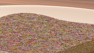
The basic idea of this shader is to scatter around wiggly lines that can be used as fibers, hairs or, like in the image below, noodles.

Each line consists of a number of segments connected end to end. Each segment is angled by a random amount relative to the previous one. Segments are not straight though, but curved by a certain amount. The parameters that control the shape of the line are illustrated below, with on the right an indication of what the basic pattern looks like:

The curved segments are implemented as quadratic splines, using routines discussed in an earlier article.

If you would like to know more about programming OSL you might be interested in my book "Open Shading Language for Blender". More on the availability of this book and a sample can be found on this page.

Code and node setup

The code is pretty straightforward. Apart from a rather long list of input parameters it is mainly concerned with calculating a list of segments for each line we want to draw (there may be more than one per cell). The main trick is in line 86, where we make certain that point p1, the point that is used to control the curvature of each segment, lies on the line line through the previous control point and the end point. This ensures that each segment joins the previous one smoothly.

#include "equations.h"

#define DOT(a,b) (a[0]*b[0]+a[1]*b[1])
#define SUB(a,b) vector(a[0]-b[0],a[1]-b[1],0)

// determine if point M is inside a rectangle with a margin
int in_rectangle(point M, point a, point b,
  vector u, float W, vector v, float linewidth){
  point A=a+linewidth*(-u-v);
  point B=b+linewidth*(u-v);
  point D=B+(W+2*linewidth)*v;
  vector AM=SUB(M,A);
  vector AD=SUB(D,A);
  vector AB=SUB(B,A);
  float dotamad=DOT(AM, AD);
  float dotadad=DOT(AD, AD);
  float dotamab=DOT(AM, AB);
  float dotabab=DOT(AB, AB);
  return (dotamad > 0 && dotamad < dotadad) && 
         (dotamab > 0 && dotamab < dotabab);
}

#define CELL noise("cell", cp, seed++)
#define CELL2 vector(CELL, CELL, 0)

shader wiggles(
  point Pos=P,
  float Scale=1,

  int Number=1,

  float Length=0.5,
  float LengthVar=0,
  float Kink=0,
  float Curl=0.2,
  float Wave=30,    // degrees
  int Steps=2,
  float StepsVar=0,

  float Width=0.02,
  float WidthVar=0,

  int Seed=0,
  
  output float Fac=0
){
  point p = Pos * Scale;
  p[2]=0;
  point ip= point(floor(p[0]),floor(p[1]),0);

  int nn=1+(int)ceil(Steps*Length);

  for(int xx=-nn; xx <= nn; xx++){
    for(int yy=-nn; yy <= nn; yy++){
      int seed=Seed;
      point cp = ip + vector(xx, yy, 0);
      for(int wiggle=0; wiggle < Number; wiggle++){
        vector start = cp + CELL2;
        start[2]=0;
        vector dir = CELL2 - 0.5;
        dir[2]=0;
        dir = normalize(dir);
          
        vector perp = vector(dir[1],-dir[0],0);
        float k=0.5 + Kink * (CELL-0.5);
        float c=Curl*(CELL-0.5);
        point p1=start+k*dir+c*perp;
        for(int step=0; step < Steps; step++){
          vector ldir = dir;
          ldir *= Length + LengthVar*CELL;
          point end=start+ldir;
          if(in_rectangle(p, start, end, dir, c/2, perp, Width+WidthVar)){
            float d,t;
            if(splinedist(start, p1, end, p, d, t)){
              float localwidth = Width+WidthVar*noise("uperlin",start,t);
              if(d < localwidth){
                Fac = (localwidth - d)/localwidth;
                return;
              }
            }
          }

          if(CELL < StepsVar){
            break;
          }else{
            p1 = end + (end - p1)*(1+noise("perlin",end)*Kink); 
            start = end;
            dir = rotate(dir, radians(Wave*noise("perlin", start)), vector(0,0,0), vector(0,0,1));
          }
        }
      }
    }
  }
}  

The only other issue that needs attention is the generation of random numbers. In each cell we need a number of them and they need to be unique. We therefore add an extra seed argument to the call to noise. However, we must take care that all those numbers are generated in a repeatable way so we reset this seed for each cell to the value provided by the Seed input. This allows us to generate unique patterns for different objects sharing the same material.
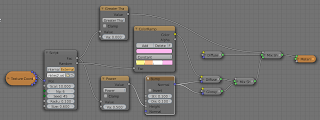
The example image at the start was created with a node setup like this:

Note that the Fac output isn't simply 1 or 0 but contains the distance to the edge of the fiber and we use that to drive a bump node (through a square root math node (power 0.5) to give it a smoothly curved appearance). We use the object info node to generate a random number because the heap of noodles consists of three separate squashed half spheres. The shader expects an integer so we multiply the random value by a million to get a unique integer.
One final node of caution: this isn't a cheap shader because calculating the distance to a spline is rather expensive. OSL is quite good at optimizing expressions but still I did dpend quite some time on optimizing the splinedist() by hand. Did did indeed shave off some small percentage but the biggest win was the conversion of all calculations to two dimensions and the test to see if we are within the bound of the control rectangle before actually checking the distance to the spline (line 72 in the code)
A final thing is that most random vectors we generate don't need the z component but OSL has no notion of 2D vectors. I rewrote that in a way that doesn't waste a third of the random values calculated (the CELL2 macro). Even with these optimizations the image with the noodles took an hour to render (200 samples on a hexacore machine). That might be a bit too much but for adding realism to a sweater (in my case that means with cat hairs all over it ;-) this might be a interesting opton.

Code availability

The code is available on GitHub. For ease of use I inlined the necessary functions from equations.h so the shader can be used as is, without external dependencies.

Sprinkles revisited

A while ago when I started this blog I created a simple shader for chocolate sprinkles and while I was reviewing comments I noticed that the code could do with some extra love.

(Whether you think this is a tasty image probably depends on you being a five year old or not :-)
There are a couple of issues with the original code:

Unnecessary functions

When the code was written OSL was lacking an implementation of the function to calculate the distance to a line segment. This is no longer the case and the functionality is provided by the three argument version of the distance() function.

Unsophisticated use of cellnoise

In the original code we added all sorts of vectors to get more than one uncorrelated cell noise value but in fact all noise variants in OSL support 4 dimensions so we can use a vector plus an additional value to get different noise values for a given cell.

Use of a deprecated function

The cellnoise() function is deprecated and we should use noise("cell", ...) in stead.

Unnecessary include

stdosl.h is automatically included by Blender already so there is no need for us to include it again.

And as a commenter mentioned, the code could do with an extra output to identify individual sprinkles so we can color them.

Code and node setup

The cleaned up code is pretty straight forward (and quite a bit shorter):

shader sprinkles(
 point Pos = P,
 float Scale = 1,
 int Np = 1,
 int Seed = 42,
 float Radius = 0.05,
 float Size = 1,
 output float Fac = 0,
 output float Random = 0
){
 point p = Pos * Scale;
 point f = floor(p);
 
 int xx,yy,np;
 vector one = 1;
 
 for( xx=-1; xx<=1; xx++){
  for( yy=-1; yy<=1; yy++){
   point ff = f + vector(xx,yy,0);
   float u=Seed;
 
   for( np=0; np < Np; np++){
    vector pd1 = 2*noise("cell",ff,u)-one;
    vector pd2 = 2*noise("cell",ff,u+1)-one;
    
    point p1 = ff + pd1;
    point p2 = ff + pd2;
    
    p2 = (p2 - p1)*Size+p1;
    
    // reduce to 2D 
    p1[2]=0;
    p2[2]=0;
    p [2]=0;
    
    float r = distance(p1,p2,p);
    if ( r < Radius ) {
      Fac = 1 - r/Radius;
      Random = noise("cell",ff,u+2);
    }
    u+=3;
   }
  }
 }
}

The node setup used to make the image at the top looks like this:

Code availability

The shader is available on GitHub. If you would like to know more about programming OSL you might be interested in my book "Open Shading Language for Blender". More on the availability of this book and a sample can be found on this page.

Some compositing experiments, mimicing black and white print

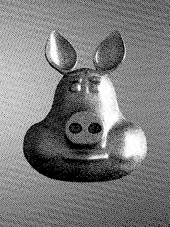
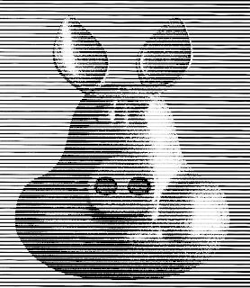
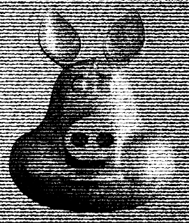
The other day I was reading about old printing techniques and I wanted to create the look and feel of screen printing with half tones and screen tones or even recreate a wood block printed look.

The approach I came up with and want to share here is pretty simple and versatile and completely implemented in compositor nodes and in the section below I show the necessary node setup. Although done in the compositor I dearly missed the possibility to create OSL nodes in the compositor because it would be nice to have some more textures to choose from.

Node setup

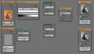
The general idea is to take a black and white version of your rendered image and combine it with some pattern. If that pattern is a smoothly varying grey scale image then it is possible compare that pattern against the b&w image and produce just black and white pixels but more of each will be produced at darker and lighter areas respectively. If that sounds confusing, bear with me it will get clearer in a minute.

The image at the start of the article was created with the node setup shown above. The image was renderered in Cycles but composited in Blender internal to be able to use textures in the compositor. This a bit awkward but not all that difficult: just set up your scene in cycles and if it renders ok, switch to bkender internal, add a new material to an arbitrary object (but don't assign it to any actual geometry) and then add a wood texture. This wood texture will give us paralel lines we can use in the compositor even though it is not actually used in any material. If you enable compositing in the post processing panel and press F12 to render, the scene will render in Cycles even though the render engine us set to internal.

In the noodle above we convert the image to black and white by plugging it into a value socket. This happens to be a colorramp node which allows use to tweak the contrast etc. The texture node refers to the wood texture we created earlier. This texture is also scaled so it will give us the line spacing we want. The real work is done in the two group nodes. These take the image and our texture, rotate the texture and do the comparison. Multiplying two versions with the lines at 90 degrees to each other give us the point pattern in the opening image.

The node group not only rotates the texture but compares it to the image. We do not simply compare whether the black & white value of the image is larger tgan that of the texture because this would give rise to horrible aliasing effects. Therefore the light orange nodes implement a smoothstep() whose smoothness is controlled by the red value node (More on this here).

Variations

Of course, in stead of multiplying two perpendicular sets if regular lines you could use any suitable pattern. The first image uses a single pattern of horizontal lines and the second image uses a marble pattern to create a wood block like appearance.

Even though you cannot uze OSL in the compositor I think it would be possible to setup two scenes in cycles, one with your image and one with just an OSL. pattern on a plane and combine these in the ckmpositor.

If you would like to know more about programming OSL you might be interested in my book "Open Shading Language for Blender". More on the availability of this book and a sample can be found on this page.

OSL Lace curtain shader for Blender Cycles, part II

In our first attempt to craft a shader that can mimic sheer fabric like lace curtains we approximated the fibers by filaments with a square cross section. In this version we see if we can work with a slightly more realistic model.
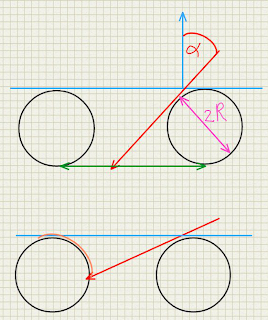
Fibers are generally not square. Their cross section more often approximates a circle. This does affect the occlusion a little bit because unlike a square the apparent cross section does not change with the angle of incidence. This means that we can approximate the transmission factor the apparent surface minus the diameter of the fiber as shown in the diagram below:

If the angle of incidence α is so large that cos(α) < 2r there will be no transmission at all.
So far this doesn't differ that much from a square cross section, however there is another phenomenon that we want to model: the sharpness of the specular reflection changes with the angle of incidence.
This happens once the angle of incidence is so large that the fiber start to occlude each other. As the occlusion increases, we see effectively a smaller segment of a circle (orange arc in left circlebin lower part of the diagram) and therefore we see less different normals. As we approach a grazing angle we effectively see just the top of the circle with normals nearly identical to the surface normal. It can be shown that the size of the circle segment we see is proportional to the angle of incidence as well.
If we compare the old and the new shader the result looks quite different:

The old equation

With new equation

Code and example node setup

The code is rather self explanatory:

shader sheet_occlusion2 (
  normal Normal=N,
  float Radius=0.05,

  output float Fac=1,
  output float Var=1
){
  // calculate angle of incidence
  float alpha = acos(dot(I,Normal));
  // treat front and back the same
  alpha = alpha > M_PI_2 ? M_PI - alpha : alpha;
  // calculate the non occluded fraction 
  Fac = cos(alpha) - 2 * Radius;
  // calculate the range of the visible normals
  if( Fac < 0 ){
    Fac = 0;
    Var = cos(alpha) / (2 * Radius);
  }
}

And the sample node setup mixes transparent shader with a non transparent shader just like before but uses the Var output to modify the shininess of the non transparent shader:

Code availability

The shader is available on GitHub. If you would like to know more about programming OSL you might be interested in my book "Open Shading Language for Blender". More on the availability of this book and a sample can be found on this page.

OSL Lace curtain shader for Blender Cycles

Lace curtains and sheer nylon stockings are partially transparent but not the way frosted glass is. Frosted glass transmits light but also diffuses it, making it almost impossible to see anything through it. Lace curtains on the other hand only obscure what's behind them if the threads of the fabric block the line of sight.

This results in the effect that you can see through lace curtains quite well if they are more or less straight and you are viewing them head on but that it is impossible to see anything behind them if seen from a glancing angle. The effect is visible quite well on the part of the curtain in front of the blue cube. Even though there isn't much specular light on the rightmost fold in front of the blue cube, it still looks brighter.

Calculating occlusion

This behavior is reminiscent of fresnel reflection but the formula is a bit different. In the diagram below the threads of the fabric are approximated by black squares. In the gap between these squares a portion is obscured from view depending on the angle α between the surface normal N and the incident ray I. The ratio between the occluded portion (pink) and the side of the square is tan(α). From the diagram it can be seen that at a certain point α is so large that the occluded portion is bigger than the gap is wide, rendering the surface effectively opaque.

Code sample and node setup

The code implementing this setup is very short and straightforward:

shader sheet_occlusion (
  normal Normal=N,
  float Radius=0.05,

  output float Fac=1
){
  // calculate angle of incidence
  float alpha = acos(dot(I,Normal));
  // treat front and back the same
  alpha = alpha > M_PI_2 ? M_PI - alpha : alpha;
  //printf("%.2f %.2f\n",alpha,tan(alpha));
  // calculate the non occluded fraction 
  Fac = 1 - Radius - Radius * tan(alpha);
}

The Fac output can be used to mix a fabric shader and a transparent shader as shown in the node setup below:

To get a pattern you could plug a black and white texture of real lace into the Radius socket.

Code availability

The shader is available on GitHub. If you would like to know more about programming OSL you might be interested in my book "Open Shading Language for Blender". More on the availability of this book and a sample can be found on this page.

Gears 2.0 (work in progres), part V, a Blender add-on

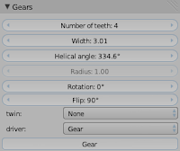
I am happy to announce that version 0.0.5 of the Gears 2.0 script is now available on GitGub. Its main new feature is the option the create involute gears, the most widely used tooth shape in modern gearing designs.

Due to ongoing backproblems my time behind a desk is severely restricted. This does mean that while the code presented in this article is actively developed, progress will be slow. This is not necessarily a bad thing because it forces me to think things through thoroughly and discuss them at length with the community before actually implementing them, which probably will lead to better code in the end.

The accuracy of the involute curve can be controlled with the steps parameter and extra space below the dedendum can be created with the fillet parameter. Likewise, extra backlash can be created between the teeth with the backlash parameter. I haven't yet printed any gears so I can't vouch for their actual mechanical behavior but for now I think this is a good start (although the shape of the fillet/undercut could be better I guess). [edit: v0.0.6 now has a shift parameter which for positive values gives a taller addendum and a shallower dedendum and for negative values the opposite. This is useful to tweak the load a gear can bear. Obviously these values should best match on adjacent gears but that is not yet done automatically]

Although I do not approximate the involute curve of the tooth with splines, this article was invaluable in getting the equations correct without trying to find it out all by myself. An example set of parameter settings is shown at the end.

Gears 2.0, a work in progress

The script is discussed on this thread on Blenderartists, feel free to comment there. It also has its own entry in Blenders upload tracker.
The code is available from GitHub, install it in the usual way from

File->User preferences->Addons->Install from file and don't forget to check the checkbox to actually activate it.

As the example below shows for a 44 teeth gear of radius 1, the fillet/undercut needs some work (it's too wide/deep) but the shape of the involute tooth itself seems ok. The read circle is the pitch radius, the blue circle the base radius (that is pitch radius * cosine( pressure angle )).

The settings to produce the gear shown above were:

3D Printing Blueprints Full Review

3D Printing Blueprints by Joe Larson, Packt Publishing
(click to go to the publisher's website)

Impressions

With literally dozens of books on 3d printing on the market yet another one has to be something of quality to be able to compete and indeed 3D Printing Blueprints does offer quality.

It has many pros:

• clear writing style
• good illustrations, in color, illustrating each step
• good coverage of concepts; modelling, material constraints, copying real life objects, designing reusable components, creating multiple component designs

Of course there are some cons:

• it's a bit short, more examples would help getting key concepts across even better
• focus is almost exclusively on makerbot and plastics (I.e home printing) while outsourcing the printing itself to an external printshop which might do materials like glass or metal is glossed over
• sometimes the illustrations are too wide for the format (I read the epub version with Aldiko on a 10" tablet so that shouldn't have occured)

What I didn't get entirely is why Blender was chosen as a modelling program. Yes it is great at modelling but many really useful features for 3d printing where not used, like assigning units (metric or imperial) or using the solidify operator, And while the introduction to basic modeling was adequate, if you keep to simple modelling a program with a gentler learning curve than Blender like for example Wings3d might have been a better choice. Of course the newest Blender revisions have addons specifically designed to help in getting your model ready for 3D printing but these are not covered in the book.

On the other hand the chapter on designing a posable teddy bear is very in depth indeed and does make use of the fairly new skin operator and some of the dynamic topology features in sculpting. It is a good introduction to skinning a stick figure and sculpting the result (and the result is cute :-).

Conlusion

So in the end, not a bad book at all if you want to give 3d printing a go and want to do more than just download and print stuff other people have designed.

Packt publishing asked me to read 3D Printing Blueprints and to write a review about it. First impressions are promising and I hope to complete reading it soon.

The software used is mainly Blender (otherwise I wouldn't discuss it here) and although the projects are focussed on printing at home on a Makerbot printer, a quick scan seems to indicate the principles will apply just as well to producing stuff at an online 3D print outfit like Shapeways.

Anyway, watch these pages for a full review somewhere next week or so.

Height to vertex weights, a Blender addon

In a previous article I presented a small script that could create a vertex group or vertex color layer with values representing the slope of faces in a mesh. The script in this article is its companion: it creates a vertex group with values representing the height (sorry no vertex color equivalent yet). I decided to make it a separate addon to keep code maintenance a bit simpler.

version 0.0.2 is now available and gives you the same possibilities as vertex colors instead of vertex weights. If you have installed the script you can find this new functionality under Paint->Height.

Terrain modelling

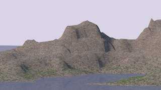
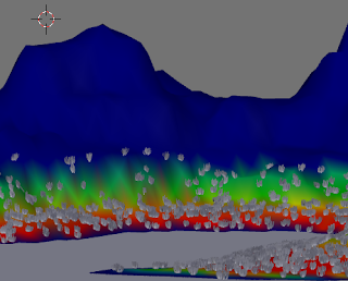
The script was created with terrain modelling in mind. You might for example want to distribute plants based on the height of a landscape mesh as shown in the (rather crude I admit) image below:

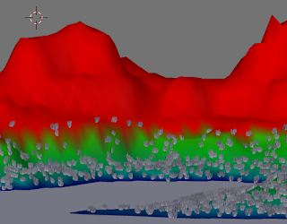
The image was created with a mesh from the ANT landscape generator to which a vertex group was added with the height addon (in weight paint mode, in the 3dview with Weights->Height). The result was this weight map:

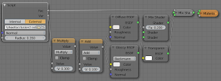
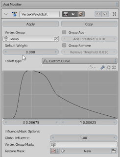
Because i wanted the grass particles to be more dense at lower altitudes, I tweaked the weights in the resulting vertex group with a vertex weight edit modifier with the following settings:

The resulting map (shown below) was then used a density map for my particle system:

Options

The scripts replaces the weights in the active vertex group to weights that represent the height or creates a new vertex group is necessary. After installation it is available in the 3dview in weight paint mode under Weights->Height It maps the chosen coordinate (x, y or z-axis) to a weight, which will be 1.0 for the largest value encountered and 0.0 for the smallest. These coordinate values are interpreted in either object (local) space or world (global) space. If the the Absolute checkbox is checked negative coordinates will be treated as positive. The mapping from [minimum,maximum] coordinate to [0,1] weight is normally linear, but may be influenced with the Power property. After mapping any values less dan Low will be set to 0, any values larger dan High will be set to 1

Code availability

All functionality of this add-on plus a lot more is now available as a convenient all-in-one add-on on BlenderMarket. It comes with an extensive PDF manual and your purchase will encourage me to develop new Blender add-ons.

The simple script shown in this article is available from GitHub and has an entry in Blenders upload tracker. There is also a BlenderArtists thread for discussing it.

Slope to vertex weights, a Blender addon part II

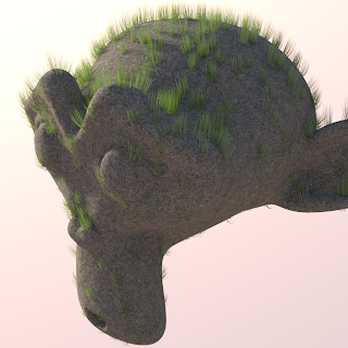
The addon's functionality was enhanced with a mirror option, to treat 'negative slopes', like those on the underside of a sphere in the same manner as positive slopes. This makes it for example possible to grow stuff on flat parts on the underside of an object while still not growing anything on the steep side as shown in the image of Suzanne (Rock material by Rasmus Seerup). Note that the default Suzanne has a ninety degree rotated mesh, so I had to rotate her in edit mode to get the slope information I needed)

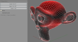
The vertex paint variant was enhanced with the option to map the calculated slope through the brush curve. This allows you the ultimate control of the weights assigned to the slope values. (Note that have to click Paint -> Slope everytime you alter the brush curve, I haven't found a way to give immediate feedback. Also the weight paint variant of this addon (which produces vertex weights instead of vertex colors and is available in weight paint mode from Weights -> Slope) does not offer this functionality itself because it is already possible to add a Bevel Weight Edit Modifier to modify vertex weights).

Code availability

All functionality of this add-on plus a lot more is now available as a convenient all-in-one add-on on BlenderMarket. It comes with an extensive PDF manual and your purchase will encourage me to develop new Blender add-ons.

The simple code shown in this article is available from GitHub snd discussed on this BlenderArtists thread. It is also followed in the Blender upload tracker. The brush curve functionality is only available for builds >= 60054 so you will have to wait for a new Blender release or build your own/download the daily build if you want to use it. The script checks for the release number so it won't crash if you have an older release.

Gears 2.0 (work in progress), a Blender addon, part IV

As you can see version 0.0.4 adds an option for an internal gear. It is a very slight enhancement, just 4 or 5 lines but it makes it possible to create the setup shown in the clip in a few seconds.

Due to ongoing backproblems my time behind a desk is severely restricted. This does mean that while the code presented in this article is actively developed, progress will be slow. This is not necessarily a bad thing because it forces me to think things through thoroughly and discuss them at length with the community before actually implementing them, which probably will lead to better code in the end.

Planetary gear workflow

• Add the first gear from the add mesh menu
• Add the second gear from the gears panel in the modifier tab by clicking the 'Gear' button,
• Select the first gear again and add another planet gear; use the rotation option to position it relative to the central gear,
• Repeat the previous step for any additional planet gear,
• Select one of the planet gear and add the outer gear. Select the 'Internal' option from the type drop down,
• Adjust the number of teeth for any of the gears to taste,
• Set some rotation keyframes for the gearhead empty to make the whole setup rotate a bit,
• Done ;-)

Slope to vertex weights, a Blender addon

As usual I enjoyed Andrew Price's tutorial on creating a cliff side quite a bit. Andrew is gifted when it comes to creating interesting Blender tutorials. However, he's first and foremost an artist. That is not meant to sound negative in any way but I observed that his solution to distributing grass along the cliff face's less steep parts was a laborious affair. Each suitable spot needed to be painted by hand.

Now this gives you ultimate control over the placement of grass tufts but wouldn't it be easier to just generate weights for a vertex group with a single clip? Of course it would and the end result can always be tweaked in weight paint mode if you would like to do so. So I wrote a small script.

The grass was done with a simple particle system that has its density set to a vertex group generated with the script.

It very much resembles my random vertex colors script so most of the work was copy and paste except for the few lines in the execute function.

The workflow is simple: after you have installed the script in the usual way, select your object and make sure you are in object mode. Then in the 3d view select Slope to vertex group from the object menu and your done.

The result is that the weights of the active vertex group have been replaced with a value representing the slope (or to be more precise the angle between the vertex normal and the object z-axis). A weight of one will be equal to a flat portion, while 0.5 will equal to a perfectly vertical part. Zero is a flat portion that is upside down. (I might change this behavior and add some options to influence the mapping range)

Code availability and discussion

All functionality of this add-on plus a lot more is now available as a convenient all-in-one add-on on BlenderMarket. It comes with an extensive PDF manual and your purchase will encourage me to develop new Blender add-ons.

The simple code shown in this article is available on GitHub and has it's own entry in Blenders upload tracker. Any comments are welcome, you might prefer this Blenderartists thread instead of this blog.

Gears 2.0 (work in progress), a Blender addon

Update: version 0.0.2 now supports out of line gears and is available from GitHub

Update: version 0.0.3 now supports worm gears and helical gears and is available from GitHub. Note that when you create a worm gear (by choosing a low number of teeth and a large helical angle, e.g. 4 and 360) you have to manually fiddle to get a fitting driven gear, automatic calculation is on my list but with 20 minutes a day (see aside) there's only so much you can do :-)


Note the two new parameters: helical angle, which is the amount of twist around the axis, and flip, which is the rotation around the axis of the gear train. The latter s needed because a driven gear is at 90 degrees relative to a worm gear.






A long time ago I wrote an addon for Blender 2.49 to create gears or cogwheels. It works quite well and it even is included as part of Blenders bundled scripts. Over the years it was maintained by other developers so it still works for Blender 2.68.

Recently Brendon Murphy (meta-androcto) asked me to look into the Gears script to resolve some bugs and while working on another plugin (the floorboard generator) I started thinking about completely redesigning the script. The most important issues prompting this redesign were:

Due to ongoing backproblems my time behind a desk is severely restricted. This does mean that while the code presented in this article is actively developed, progress will be slow. This is not necessarily a bad thing because it forces me to think things through thoroughly and discuss them at length with the community before actually implementing them, which probably will lead to better code in the end. Nevertheless, version 0.0.1 is available (see below) although those few lines of code took over two weeks to code (and a large part was borrowed from other addons :-)

Bmesh

When the script was written, Bmesh support in Blender was not even a glimmer of an idea so the code that creates the actual geometry isn't exactly elegant. Redesigning for Bmesh not only makes for cleaner code but is also a personal incentive to learn more about this Api, which isn't always completely documented (return values from operators are often dictionaries with all kind of geometry information yet the different values they contain are often not described in full) but which is both powerful (supporting complex operations like duplication and extrusion) and fast (implemented in C/C++, Python is just a thin wrapper).

Parameterization

When I was working on the floorboard generator Marcatore showed me a design by DragonLee to make options persistent. The original gears addon suffers from the same affliction as many other addons in that once the object is created you cannot easily tweak it. You can of course manually alter the mesh but the option sliders are gone from the toolbar as soon as the mesh is manipulated in any way. What we really want is the possibility to tweak the options even after saving and reloading the .blend and this exactly what DragonLee's method makes possible, paving the way for truly parametric objects.

Animation suport

Configuring a rig or drivers to let one cogwheel drive a bunch of other cogwheels is not that simple and rather time consuming. So the new design should feature drivers and keyframes that allow for instant animation, which then of course may be adapted to your specific needs.

User friendliness

Many addons are not written with user friendliness in mind and I am guilty of this sin as well. There are basically two solutions to this problem (and they can be used in parallel): One, use your own addon extensively, asking yourself with each mouseclick if it is necessary and with each option you introduce if its description is clear and relevant, and two, interact with the community, for example on Blenderartists. Ask what features they miss and ask explicitely how usability might be improved. Do this early on, not when your script is almost finished, although it should already be quite usable when you introduce it, otherwise no one will try it out.

With those considerations in mind I present you:

Gears 2.0, a work in progress

The script is discussed on this thread on Blenderartists, feel free to comment there. It also has its own entry in Blenders upload tracker.
The code is available from GitHub, install it in the usual way from

File->User preferences->Addons->Install from file and don't forget to check the checkbox to actually activate it.

Workflow

The workflow in general is very simple:

• Add the first gear that will drive the rest of the mesh with Add->Mesh->Add Gear
• Locate the Gears panel in the modifiers tab of the properties
• Add as many gears as you need by clicking Gear (the button at the bottom of the panel)
• Select each gear in turn and alter its properties as needed

At this point you will have an animated gear train. You can step through the frames to see it move. At the location of the first gear is a spherical empty (called GearHeadEmpty) which can be moved and rotated to position the whole gear assembly in any way you like.
To recreate the gears in the opening image/video go through the following steps:

Add the first gear

Click Add->Mesh->Add Gear

Add four additional gears

Click Gear four times in the Gears panel in Modifiers tab of the Properties

Give the first gear 20 teeth

Select the first gear and adjust the Number of teeth to 20

Give the second gear 6 teeth

Select the second gear and adjust the number of teeth like you did for the first gear

Give the third gear 20 teeth

Just like the first and second gears

Give the fourth gear 6 teeth

Should be familiar by now

Give the fifth gear 20 teeth

You should be able to do this with your eyes closed by now :-)

Twin the second gear to the first

Select the second gear and choose Up from the Twin dropdown. The gear will move to the location of first gear, slightly shifted along the z-axis and its animated rotation will be identical to that of the first gear, all as if both gears are connected to the same gear axis.

Twin the fourth gear to the third

Select the fourth gear and choose Up from the Twin dropdown like you did for the second gear.

Done!

Step through the frames or press ctrl-A to see the gear assembly move.

Road map (provisional)

Whatever will be developed depends of course on the feedback I get but my personal list features the following items (in no particular order):

• rotate gear out of line, to allow a more varied placement of the gears
• parameterization of tooth (size, margin, angle)
• parameterized depth, taper and twist (to make conical and helical gears)
• spokes + axes
• uv-map
• material slots w. simple cycles material.[gear, spoke, axis]
• worm gear?

Generate floor boards quick and easy, part VI

This version (0.0.8) of the floor board generator adds options to add twists and hollow curvature to the individual planks. This is useful when creating floors in older houses and its more subtle simply rotation planks. All the options are now visually grouped as well to aid the user in locating related options.

The floor board generator is documented in several blog articles. Apart from the one you are reading now, the series consists of:

Part I

initial version

Part II

random uv-coordinates

Part III

random vertex colors

Part IV

additional options

Part V

randomization

The latest version of the code is available from GitHub and is tracked in the Blender Extensions tracker (although most of the discussion is in this BlenderArtists thread.

An example (with a flat material to emphasize the subtle curvature) is shown below (click to enlarge):

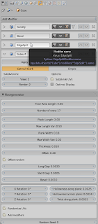
The option values used to create the image are shown in the next image. Note that for illustrative purposes we made the gaps between the planks quite large:

Parameterization

The biggest change in this version was already visible in the image above: parameters no longer appear in the toolbar but in the FloorBoards section of the modifier options. This is not only a visual change but it actually means that even after savinf the .blend file all relevant parameters are retained along with the abject and can be tweaked at any time. (Thanks floric for the code adaptation and DragonLEE for the original idea)

Generate floor boards quick and easy, part V

This version (0.0.7) of the floor board generator adds options to add small random rotations to the individual planks. This is useful when creating floors in older houses. All the options are now visually grouped as well to aid the user in locating related options.

The floor board generator is documented in several blog articles. Apart from the one you are reading now, the series consists of:

Part I

initial version

Part II

random uv-coordinates

Part III

random vertex colors

Part IV

additional options

The latest version of the code is available from GitHub and is tracked in the Blender Extensions tracker (although most of the discussion is in this BlenderArtists thread.

An example (with exaggerated values for the rotations) is shown below (click to enlarge):

The option values used to create the image are shown in the next image. Note that for illustrative purposes we made the gaps between the planks and the random rotation values quite large:

Generate floor boards quick and easy, part IV

In a previous post I added some extra functionality to the floor board generator and based on user feedback and code contributions there are now some more options:

• the offset can now be random for each individual row of planks (thanks Alain for your contribution)
• adding modifiers is now optional (but on by default)
• adding random offsets to the uv-map for each plank is now optional (but on by default)

Code availability

This new version (0.0.6) is available for download from GitHuband is tracked in the Blender extensions tracker as well.

Random Vertex Colors, a simple addon

In a previous article I presented an addon to generate a floor board with individual planks. Each individual plank was adorned with a random vertex color that can be used to create materials with random color variations for each face.

When working with the Ivy Generator recently I wanted this same feature and indeed my own space tree addon could benefit from this as well, because just like IvyGen it generates a single mesh object with a face. for each leaf. So I decided to separate this functionality from the floor board generator so it can be used in different situations.

Once the addon is installed it can be used on any mesh object when in vertex paint mode as shown below:

It will replace the vertex colors of the active vertex color layer with colors that are random but equal for each face. In Cycles vertex colors can be accessed with an attribute node, an example node setup can be found in the article on the floor board generator referred to at the start of this article.

Code availability

All functionality of this add-on plus a lot more is now available as a convenient all-in-one add-on on BlenderMarket. It comes with an extensive PDF manual and your purchase will encourage me to develop new Blender add-ons.

The simple code shown in this article is available for download at GitHub and is uploaded to the upload section of Blender extensions tracker so if you find bugs you may post them there as well.

[2016 Feb 7] The version currently in GitHub is much faster for large meshes because it uses Numpy. Check this article to see why.

Voronoi playtime, some Cycles OSL secrets

This article now has a follow up that shows how to implement different distance metrics.
Members over at BlenderArtists wondered what it would take to get the diversity of voronoi textures back in Cycles which are present in Blender Internal. Well, the functionality is available but hidden in an OSL include file, so it takes a very simple OSL script node to get at it.
The example below is a Voronoi Crackle textures (basically the distance to the second closest point minus the distance to the closest point):

The node setup for this image is shown below.

Code

The code is quite simple. It utilizes the node_texture.h include distributed with Blender. Its outputs are the distances to the four closests points.

#include "node_texture.h"

shader Crackle(
  point p = P,
  output float Fac1 = 0,
  output float Fac2 = 0,
  output float Fac3 = 0,
  output float Fac4 = 0
){
  float da[4];
  point pa[4];

  voronoi(p, "Distance Squared", 0, da, pa);
  
  Fac1 = da[0];  
  Fac2 = da[1];  
  Fac3 = da[2];  
  Fac4 = da[3];  
}

Mind you, there is a lot more in the include (it is in the scripts\addons\cycles\shader directory of you Blender distribution), it even sports a voronoi_Cr function which does more or less the same as the node setup below, but this node is a bit more versatile for your experimentation :-) The only drawback is that we cannot define anything in the make up of the node ohter than its input and output sockers, so it is not possibly to define a nice drop down with for example distance metrics in OSL. (We could use an integer socket to switch, but that feels clunky).

Example node setup

The image at the start of this post was created with the following node setup:

Generate floor boards quick and easy, part III, vertex colors

A member at BlenderArtists really wanted to apply a random material to each individual plank. Now Cycles can generate a unique random number for each object but not for each face within an object so another trick was needed. I therefo , added a vertex color layer with a unique color for each plank. Vertex color layers may be accessed from Cycles with an attribute node as shown in the node setup below:

In the example we use the color directly but of course it can be treated as a random value to control some specific material property ad well, that is left as an exercise for the reader.

Code availability

The code is available on GitHub but as I hope to promote it to the Contrib repository one time, it's also in the Blender upload tracker.

Irregular stone patterns in OSL, a first attempt

On the BlenderArtists forum a member was analyzing irregular stone walls and posed the interesting question: does this resemble a tree pattern and can it be done in OSL? Quite a lot of thinking and tinkering is needed for a full solution put in this post we explore some of the basic requirements.

Irregular stone patterns

A sample pattern with primary colors, Mondrian eat your heart out :-)
The sample image shows that we have generated a pattern consisting of rows with different heights, each consiting of stones of varying width. Additionally, some stones within a row are further split horizontally. The code to generate the pattern is shown below:

shader stones(
  point p = P,
  vector Scale = 1,
  float w = 0.02,
  float s = 2,
    
  output float Fac = 0
){
  point Pos = p * Scale;
  
  float bot = floor(Pos[1]-1)+cellnoise(Pos[1]-1);
  float lev = floor(Pos[1])+cellnoise(Pos[1]);
  float top = floor(Pos[1]+1)+cellnoise(Pos[1]+1);

  if( Pos[1] < lev ){
    Pos[0] += s*cellnoise(Pos[1]);
  }else{
    Pos[0] += s*cellnoise(Pos[1]+1);
  }
  float left = floor(Pos[0]-1)+cellnoise(Pos[0]-1);
  float mid = floor(Pos[0])+cellnoise(Pos[0]);
  float right = floor(Pos[0]+1)+cellnoise(Pos[0]+1);
  if( 
    ((Pos[0] > left+w) && ( Pos[0] < mid - w )) 
    || 
    ((Pos[0] > mid+w ) && ( Pos[0] < right - w))
  ){
    if( 
      ((Pos[1] > bot+w) && ( Pos[1] < lev - w )) 
      || 
      ((Pos[1] > lev+w ) && ( Pos[1] < top - w))
    ){
      int stoneindex=0;
      float seeda = left;
      float seedb = bot;
      float bounda = mid;
      float boundb = lev;
      
      if( Pos[0] > mid ){ stoneindex += 2; seeda = mid; bounda = right; }
      if( Pos[1] > lev ){ stoneindex += 1; seedb = lev; boundb = top; }
      int pattern = (int)floor(cellnoise(seeda,seedb)*4);
      if( pattern == 0 ){
            // horizontally halved
            float nlev = (seedb + boundb)/2;
            if( (Pos[1] > nlev - w) &&  (Pos[1] < nlev + w) ){
              Fac = 0;
            } else {
              Fac = cellnoise(vector(seeda,seedb,Pos[1]>nlev));
            }
      } else {
        Fac = cellnoise(vector(seeda,seedb,-1));
      }
    }
  }
}

(The code is also available on GitHub.)

Sample node setup

The example image at the top of this article was made with the following node setup (click to enlarge)
:

Further work

Obviously we need more sub patterns for the individual stones and add some distortion to the underlying coordinates to make really random stones. It would probably also be a good idea to vary the spacing between the stones and use the output value to drive displacement and bump maps and the code could certainly do with a bit of cleanup but I thinks this approach is at least shows promiss.