Add-ons and more

Upgrading Blender add-ons from 2.79 to 2.80, part 3

While porting my add-ons from Blender 2.79 to 2.80 I encounter all sorts of compatibility issues that I report on from time to time in this blog. Some of those of issues are minor but others go deeper and might take quite some effort to fix.

In previous articles I listed a fair number of issues (1, 2) but the good news is that the number of new issues that pop up is diminishing. Last week's batch is rather small:


  • context.user_preferences becomes context.preferences. That is fairly easy to fix but unfortunately this could break stored preferences as well since they might contain references to this attribute in the set itself (A stored preference or preset is executable Python code that basically sets all sorts of variables)


  • BVHTree.fromobject and related functionality was broken but is now fixed. Thanks to very rapid follow up by Blender dev Bastien Montagne! Note that even though the bug is fixed, the signature of this function (and related ones) has changed: It no longer takes a Scene argument but a Depsgraph argument.


  • context.area.header_text_set(None) must be used instead of context.area.header_text_set("") to restore the default menu. This is not a big thing but if you forget you get an empty taskbar.


IDMapper ported to Blender 2.80


IDMapper has now been ported to Blender 2.80 and is available from BlenderMarket.

There were a fair number of bumps along the road with regard to some parts of the Python API so be aware that Blender 2.80 is still in beta and you might still encounter some difficulties!

Blender add-on: mesh to heightmap

Sometimes it would be convenient to convert a mesh to a heightmap. If you would have a heightmap available, you could flatten your mesh geometry and add a displacement modifier or material with micro displacement instead.

This has many possibilities, including post processing the heightmap in an external program or using adaptive subdivision to reduce geometric complexity where it isn't needed. Therefore I created a small add-on that does just that: Given a mesh that is uv-mapped it creates a new image which contains the z coordinates as grey-scale values.


(original mesh on the left, flattened mesh with map added via a displacement modifier on the right)


(a uv-mapped plane with a single face plus an adaptive subdivision modifier)

Limitations

The add-on will map the object z-coord to a grey-scale value, so this will only work properly on rectangular landscapes, not for example spherical ones. The whole range of z-coordinates present will be mapped to the range [0,1].
You can generate any size map you like, even non-square ones, but the map should be smaller than twice the number of vertices in any dimension, and if you select a map size larger than the number of vertices in a dimension you should check the interpolate option to avoid black lines.
For example, if you have generated a 128 x 128 landscape, you can generate a 128 x 128 map, or any smaller one, but for bigger ones up to 256x256 you need to check the interpolate option.
If you need even bigger maps, generate one that fits will and resize in an external program like Gimp.

The add-on is not super robust and will fail if the mesh has no active uv-map and also when the uv-coordinates are outside the range [0,1] (which is perfectly legal but either scale your uv map before generating the heightmap or adapt the add-on)

Relevant bits of code

For those interested in the inner workings: 

  • line 05: create a new image
  • line 08: initialize the image to an opaque all black
  • line 11: get all uv coordinates from the active uv-layer into a numpy array
  • line 16: get all vertex coordinates into a numpy array
  • line 21: get all vertex indices from the loops. Note that loops and uv-coordinates are aligned, i.e. eery loop has a uv coordinate in a uv-layer
  • line 24: scale/map the z component of the coordinates to the range [0,1]
  • line 31: map uv-coordinates to image pixel coordinates
  • line 35: for every uv value and height, assign the corresponding pixel rgb value. We do not change the alpha. Note that we do this for every loop, not just for every vertex, so this is very inefficient: a typical all-quad mesh contains four loops for every vertex! However, this is fast enough in practice so I didn't bother to optimize
  • line 38: optional interpolation. We determine the missing pixel coordinates and then interpolate those values from the immediate neighbors. 
  • line 50: assign the calculated grey-scale values to the pixels. Note that copying a complete array like we do here is rather fast but would we have done it by indexing the pixels attribute pixel by pixel this would have been prohibitively slow.

 def execute(self, context):
  mesh = context.active_object.data
  width, height = self.width, self.height

  im = bpy.data.images.new("Heightmap",
                    height, width, float_buffer=True)

  hm = np.zeros((width, height, 4), dtype=np.float32)
  hm[:,:,3] = 1.0

  uvlayer = mesh.uv_layers.active.data
  uv = np.empty(len(uvlayer)*2, dtype=np.float32)
  uvlayer.foreach_get('uv',uv)
  uv.shape = -1,2

  co = np.empty(len(mesh.vertices)*3, dtype=
  np.float32)
  mesh.vertices.foreach_get('co', co)
  co.shape = -1,3

  vi = np.empty(len(mesh.loops), dtype=np.int32)
  mesh.loops.foreach_get('vertex_index',vi)

  z = co[:,2][vi]
  zmax = np.max(z)
  zmin = np.min(z)
  zd = zmax - zmin
  z -= zmin
  z /= zd

  uv[:,0] *= height-1
  uv[:,1] *= width-1
  uv = np.round(uv).astype(np.int32)

  for h,xy in zip(z,uv):
   hm[xy[1],xy[0],:3] = h

  if self.interpolate:
   uniq0 = np.unique(uv[:,0])
   uniq1 = np.unique(uv[:,1])
   missing0 = np.setdiff1d(np.arange(height, 
                             dtype=np.int32), uniq0)
   missing1 = np.setdiff1d(np.arange(height,
                             dtype=np.int32), uniq1)
   for y in missing1:
    hm[y,:] = (hm[y-1,:] + hm[y-1,:])/2
   for x in missing0:
    hm[:,x] = (hm[:,x-1] + hm[:,x+1])/2

  im.pixels[:] = hm.flat[:]

Availability

The add-on is available from my GitHub repository (right click on link and select Save As ... or equivalent for your browser). After installing and enabling the add-on, a new menu item Object -> Mesh2Heightmap will be available in the 3d-view in object mode.

Upgrading Blender add-ons from 2.79 to 2.80, part 2

In the first part of this series on porting add-ons from 2.79 to 2.80 I promised to keep notes on issues that might pop-up so here is my second batch:


  • scene.objects.active is no longer available. Use context.active_object. This is due to working with collections,
  • no bl_category, so you cannot decide where your Panel will be located in the Toolbar. This is too bad, but maybe I don understand this completely,
  • the bgl module does not support direct mode at all (not even as an option). This hurts really bad. Yes the new , modern OpenGL capabilities are what we all wished for but porting the old stuff to the new is far from trivial,
  • BVHTree.FromObject() expects a Depsgraph not a scene. This is a breaking change. The relevant Depsgraph is available from context.depsgraph,
  • scene.ray_cast() expects a view_layer to determine what is visible in the scene. Again a breaking change related to the previous one. The relevant view_layer is available from context.window.view_layer,
  • Lamps are now called Lights, this affects object.type ('LIGHT') as well as bpy.data.lights,
  • Color() constructor always expects 3 values, but the .color attribute in a vertex color layer is 4 items (RGBA). Like the next item on this list this might have been present in 2.79 already but just comes to light now that I am porting add-ons,
  • The name of a module may not contain -  (i.e. a dash or minus sign) or install will silently fail (might have been the case in 2.79 too)

WeightLifter ported to Blender 2.80


WeightLifter has now been ported to Blender 2.80 and is available from BlenderMarket.
Porting this add-on was a bit more work than porting NodeSet Pro, so be aware that Blender 2.80 is still in beta and you might still encounter some difficulties!

NodeSet Pro ported to Blender 2.80


NodeSet Pro has now been ported to Blender 2.80 and is available from BlenderMarket.
Porting this add-on has been fairly easy but be aware that Blender 2.80 is still in beta so you might encounter difficulties!

Upgrading Blender add-ons from 2.79 to 2.80

i have started research into upgrading my (commercial) add-ons from 2.79 to 2.80. in documenting what i encounter, i hope i can spare people some frustrations and learn something about add-ons in general. i didn't start earlier, partly because i had some other stuff to do but mainly because the Python API needed to be finalized and more or less stable: with many add-ons to consider for an upgrade starting when everything is still in flux would run the risk of wasting a lot of time.

Expectations

the Blender developers provided some documentation in the API changes in in a short document. Unfortunately, quite a few of them are breaking changes, i.e. the have to be changed in order to work at all. Many of these changes impact every add-on, like no longer having a register_module() utility function while some others apply mainly to math heavy add-ons, like the use of the @ operator for matrix multiplication. Unfortunately quite a few of my add-ons are math heavy so i will probably need to spend quite some time on this.

Annoyances

the Blender devs decided it was a good idea to force all keyword parameters to actually use those keywords. And indeed this will prevent accidentally using a positional argument as a keyword argument and aid in readability. This is a Good Thing™. However it is bloody annoying that layout.label() is affected by this, which I use a lot which just a single text argument ...
The price for biggest annoyance however goes to the mandatory change that forces class variables that are initialized with a call to some sort of property function like an Operator with for example a size = FloatProperty(name="size") property, to a type annotation like size: FloatProperty(name="size")
A small change it may seem but properties are everywhere so it is a lot of work. And although i read the PEP thoroughly, I fail to see the advantage. I'd rather hoped the devs would concentrate on things that change because of Blender's new structure, like collections and viewport related things, than on this new Python fad ...

Upcoming

I am just starting the research on converting my add-ons but you can expect a couple of articles the next couple of months with hopefully some useful findings.

Blender Market black friday sale

Blender Market will feature a black friday / cyber monday sale this weekend. Many products will be 25% off, including of course all my add-ons ;-) 
So if you were thinking about TextureWatch, NodeSet Pro, Ortho, IDMapper, WeightLifter or even SpaceTree Pro, this will be your change to get them at a nice discount in my BlenderMarket shop.
Many other creators of add-ons as well as models, shaders etc. will participate so be sure to visit BlenderMarket's home page as well.

Change the radius and type of metaball elements

A couple days ago I published a tiny add-on to manipulate the attributes of all meta elements inside a metaball. Because it can be helpful to change the radius of an individual element after is is created I added a small panel that lets you do that (because it is currently only exposed in a Panel in the Ctrl-N sidebar which is not logical).

I have submitted a patch that is now included in the master and 2.8 branches but for now I keep this extra panel in for people who are not able to use the latest built.

The Panel looks like this:

That might not be the prettiest way to do it but it gets the job done. Note that it will change the radius of the active metaelement (just like the other attributes), not of the selected element(s). This is inconsistent with editing regular meshes but unfortunately not something I can change.

Metaelement type

In some situations it might be useful to change the type of all metaelements as well, so I added that option to the operator:
Not that we also have a 'Keep´ option (the default) that will let you scale just the other attributes without changing the element type.

Code availability

The updated add-on is available from my GitHub repository.

Blender addon: scale attributes of metaball elements

Blender has had some support for metaballs since ages yet the amount of development love they get is not much: some attributes of the individual metaball elements are not exposed to the Python API (like select) and/or are not exposed in the interface. It is for example not possible to change the initial radius of an element once created and it is also not possible to change the stiffness or size attributes for any element but the active one (the S key scales the position of the elements).

This is quite annoying because for some voxel based visualizations metaballs are actually quite nice and the implementation in Blender is reasonably fast too. In order to remedy some of the missing featues I created a small add-on that allows you to scale the radius, stiffness and size attributes of all elements of a selected metaball.

Example

Once installed the operator is available in edit mode under the Metaballs menu. When selected it offers the attributes in the operator panel in your 3d-view toolbaar (press ctrl-T if the toolbar is not visible)

Note that scaling any of those attributes will affect all elements in the metaball object because as explained earlier the select status of individual elements is not exposed to the Python API so unfortunately we have no way of limiting the activity.

Code availability

The code is available on my GitHub repository (you might need to right-click and select File->Save As ... or equivalent depending on your browser)

Extended Voronoi Texture support in Blender

A long time a go I reported on my efforts to get a more versatile Voronoi texture node in Blender but this effort never led to actual inclusion of the code.

But all of a sudden there has been some interest again and now we have extended Voronoi functionality in the Voronoi texture node! And of course Pablo in his unique enthusiastic style did a nice demo of it as well check out the video.

The new functionality is available in the latest build of 2.79 and presumably in the 2.8 branch too. Note that in my original patch I included Voronoi crackle as well, but that is not available in the new node itself. However since Voronoi crackle is simply the difference between the distance to the 2nd closest and the 1st closest point, this popular pattern is super easy to implement now with the following noodle:


Finally an easy way to generate lizard scales :-)


Blender Market 2018 fall sale

Blender Market will feature a sale from September 19 - saturday September 22. Many products will be 25% off, including of course all my add-ons ;-)
So if you were thinking about TextureWatch, NodeSet Pro, Ortho, IDMapper, WeightLifter or even SpaceTree Pro, this will be your change to get them at a nice discount in my BlenderMarket shop.
Many other creators of add-ons as well as models, shaders etc. will participate so be sure to visit BlenderMarket's home page as well.

Add-on: export a mesh as an OpenGL display list

Ok, I know this will only benefit very few people but that doesn't stop me from sharing :-)

A cloud of OpenGL Suzannes

What is it?

A tiny add-on that exports a small Python file containing OpenGL code to display a mesh.

What is it good for?

Blender has OpenGL bindings available for use in Python scripts. You can use these OpenGL drawing commands to display for example overlays over your 3D view with a draw handler.
If you would want to draw some sort of complex object you would have to recreate it using glVertex3f() calls which is a lot of work as soon as the model is more than a few vertices. This add-on generates the code for you in the form of a function that creates a display list.

How does it work?

When you select File -> Export -> Export mesh as OpenGL snippet it will open a file dialog and then it will write Python code to the selected file.
It will write the vertex coordinates (in object space) and the vertex normals of the active object. It will triangulate the mesh internally before writing it. There is currently no check if there is an active object or that the active object is a mesh.

What does the resulting Python code look like?

The export for a plain Suzanne mesh looks like this:

import bgl

def Suzanne():
 shapelist = bgl.glGenLists(1)
 bgl.glNewList(shapelist, bgl.GL_COMPILE)
 bgl.glBegin(bgl.GL_TRIANGLES)
 bgl.glNormal3f(0.9693,-0.245565,-0.011830)
 bgl.glVertex3f(0.4688,-0.757812,0.242188)
 bgl.glNormal3f(0.6076,-0.608505,-0.510393)
 bgl.glVertex3f(0.5000,-0.687500,0.093750)
 bgl.glNormal3f(0.8001,-0.599853,-0.002850)
        ... lots of calls omitted ...
 bgl.glVertex3f(-0.5938,0.164062,-0.125000)
 bgl.glEnd()
 bgl.glEndList()
 return shapelist

That code is so old fashioned, why?

If you ask any questions on forums like stack-overflow about older versions of OpenGL (and old in this context essentially means anything before OpenGL 3.0) you will be told over and over again that you shouldn't use it and that investing time in it is wasteful or even stupid.
You will have to live with that :-)
The fact is that even though Blender certainly runs on newer versions of OpenGL, the Python bindings it provides are based on version 2.1 and I am not sure when that will change. And yes, even 2.1 supports stuff like vertex arrays but those are quite cumbersome to use, not documented in the Blender Python API any in many situations overkill and not really a speed improvement: If all you want is some fancy overlay, using a compiled display list is pretty fast.

Where can I download it?

The add-on is available on GitHub.

Blender add-on: TextureWatch

I am happy to announce that yesterday I published my new TextureWatch add-on on Blendermarket.

As illustrated in the video, TextureWatch is a small add-on to automatically synchronize textures used in your .blend file if they change on disk. This simplifies working with external programs like Gimp or Substance Painter because TextureWatch can automatically update those textures when you save your files without the need to go through all images inside Blender one by one and selecting reload. This saves time as well as guarantees consistency.


If you find this useful you might want to take a look at my BlenderMarket store.

Graswald vs. Grass Essentials

I recently bought the Graswald add-on because the sample images looked really good and the collection of plant species, variations and leaf debris on offer was quite extensive.

A couple of years ago I also bought Grass Essentials and although that was (and is) is fine collection of grasses and weeds too, I always found it rather difficult to get naturalistic looks. Both products have options to change things like the patchiness or wetness of the plants but I feel that Graswald, being an add-on*) with all the configurable options in a toolbar panel is far easier to work with and offers some extra possibilities, like integration with weight painting for distribution and length as well as aging a percentage of the plants .

*) It is also available as an asset library without the add-on at a slightly lower price.

Example


To show you what I mean I spent some time trying to recreate a patchy grass field consisting mainly of Kentucky Rye grass sprinkled with lots of dandelions. It took me about 10 minutes to set up the Grasswald patch on the left and although the time it took to set up the Grass Essentials patch on the right was about the same, I lost some time because although Grass Essentials does have dandelion flowers and seed-heads, it does not have a particle system to represent the actual dandelion plant leaves, so I finally substituted those with plantain to get at least some leaves showing.

(click to enlarge. Image rendered in Cycles with 1000 samples, filmic color management at medium high contrast and lit by a single HDRI backplate from HDRI Haven. The ground texture barely visible below the plants was a simple dirt texture created in Substance Painter. Note that Grass Essentials bundles several good dirt textures as well.)

Conclusion


Now everybody knows I not much of an artist and probably with some extra time the Grass Essentials version could be made to look more varied and patchy but for me the ease of use and the quality of the end result speaks for itself. Given this quality and ease of use combined with the slightly lower price, Graswald easily wins out on value for money.

[These opinions are my own. I am no way affiliated with either Graswald or Grass Essentials and did pay for both products myself.]

Raytracing concepts and code, part 11, antialiasing


This is an article in a multipart series on the concepts of ray tracing. I am not sure where this will lead but I am open to suggestions. We will be creating code that will run inside Blender. Blender has ray tracing renderers of course but that is not the point: by reusing Python libraries and Blender's scene building capabilities we can concentrate on true ray tracing issues like shader models, lighting, etc.
I generally present stuff in a back-to-front manner: first an article with some (well commented) code and images of the results, then one or more articles discussing the concepts. The idea is that this encourages you to experiment and have a look at the code yourself before being introduced to theory. How well this works out we will see :-)

So far the series consists of the several articles labeled ray tracing concepts

Anti aliasing

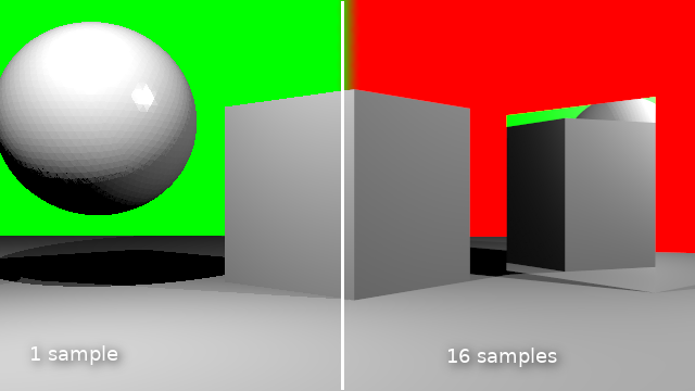
If we want to diminish the jagged look of edges in our rendered image we can sample a pixel multiple times at slightly different positions and average the result. In this article I show the code to do this.

Code

Once we know how many times we want to sample a pixel we have to calculate our camera ray as many times but with slightly shifted coordinates and then average the result. If we take the original direction of the camera ray to point into the exact middle of an on screen pixel, we have pick a point in the square centered around this point.
For this we first calculate the size of this square (line 9 and 10). Then as before we calculate each pixel but we repeat this for every sample (line 14). We keep the sum of all our samples in a separate buffer sbuf (defined in line 5, the addition is in line 23). We still want the final buffer that will be shown on screen to represent the averaged color we calculated so far, so in line 15 we update a whole line of pixels to represent the current average.
We also invert the line above it (line 16,17) so we have some visual feedback of where we are when we are updating the buffer. This is useful to keep track as with increasing samples the contribition gets smaller and might be hardto see.
Finally we yield the percentage of samples we calculated so far.
Note that the vdc() function returns a number from a Van der Corput sequence. I have not shown this function and you could use uniformly distributed random numbers instead (shown in the line that is commented out) in stead of these quasi random numbers, but these should give better results. The reasoning behind this is out of scope of this article but check Wikipedia for more on this.
def ray_trace(scene, width, height, depth, buf, samples, gi):     

    ... indentical code left out ...

    sbuf = np.zeros(width*height*4)
    sbuf.shape = height,width,4

    aspectratio = height/width
    dy = aspectratio/height
    dx = 1/width
    seed(42)

    N = samples*width*height
    for s in range(samples):
        for y in range(height):
            yscreen = ((y-(height/2))/height) * aspectratio
            for x in range(width):
                xscreen = (x-(width/2))/width
                #dir = Vector((xscreen + dx*(random()-0.5), yscreen + dy*(random()-0.5), -1))
                dir = Vector((xscreen + dx*(vdc(s,2)-0.5), yscreen + dy*(vdc(s,3)-0.5), -1))
                dir.rotate(rotation)
                dir = dir.normalized()
                sbuf[y,x,0:3] += single_ray(scene, origin, dir, lamps, depth, gi)
            buf[y,:,0:3] = sbuf[y,:,0:3] / (s+1)
            if y < height-1:
                buf[y+1,:,0:3] = 1 - buf[y+1,:,0:3]
            yield (s*width*height+width*y)/N
When we call our new ray_trace() function we have to determine the number of samples first. Blender provides two properties from the render context for this: scene.render.use_antialiasing and scene.render.antialiasing_samples. For some reason that last one is a string, so we have to convert it to an int before we can use it:
    def render_scene(self, scene):

    ... indentical code left out ...

        samples = int(scene.render.antialiasing_samples) if scene.render.use_antialiasing else 1
        for p in ray_trace(scene, width, height, 1, buf, samples, gi):

    ... indentical code left out ...

Now we could make the whole existing anti-aliasing panel available by again adding our engine to the COMPAT_ENGINES attribute but because it had lots of options we don't use we create our own panel with just the properties we need (something we might do later for other panels as well):
from bpy.types import Panel
from bl_ui.properties_render import RenderButtonsPanel

class CUSTOM_RENDER_PT_antialiasing(RenderButtonsPanel, Panel):
    bl_label = "Anti-Aliasing"
    COMPAT_ENGINES = {CustomRenderEngine.bl_idname}

    def draw_header(self, context):
        rd = context.scene.render

        self.layout.prop(rd, "use_antialiasing", text="")

    def draw(self, context):
        layout = self.layout

        rd = context.scene.render
        layout.active = rd.use_antialiasing

        split = layout.split()

        col = split.column()
        col.row().prop(rd, "antialiasing_samples", expand=True)

Code availability

The revision containing the code changes from this article is available from GitHub.


Raytracing concepts and code, part 10, showing progress


This is an article in a multipart series on the concepts of ray tracing. I am not sure where this will lead but I am open to suggestions. We will be creating code that will run inside Blender. Blender has ray tracing renderers of course but that is not the point: by reusing Python libraries and Blender's scene building capabilities we can concentrate on true ray tracing issues like shader models, lighting, etc.
I generally present stuff in a back-to-front manner: first an article with some (well commented) code and images of the results, then one or more articles discussing the concepts. The idea is that this encourages you to experiment and have a look at the code yourself before being introduced to theory. How well this works out we will see :-)

So far the series consists of the several articles labeled ray tracing concepts

Progress

The bits of code we show in this article have less to do with raytracing per se but do show off the options to indicate progress in Blender's RenderEngine class. Not only gives this some visual feedback when rendering takes long, it also gives the user the opportunity to cancel the process in mid-render.

Code

First we change the ray_trace() function into a generator that returns the y-coordinate after every line. This is accomplished by the yield statement. So now the function doesn't allocate a buffer itself but it takes a buf argument.
def ray_trace(scene, width, height, depth, buf):     

    ... identical code left out ...

    for y in range(height):
        yscreen = ((y-(height/2))/height) * aspectratio
        for x in range(width):
            xscreen = (x-(width/2))/width

            ... identical code left out ...            

        yield y
The render_scene() is changed too: it allocates a suitable buffer and then iterates over every line in the render result as it gets rendered (line 9). It then calls the update_result() function of RenderEngine class to show on screen what is rendered so far (line 12). It also calculates the percentage that has been completed and signals that as well (line 14).
    def render_scene(self, scene):
        height, width = self.size_y, self.size_x
        buf = np.ones(width*height*4)
        buf.shape = height,width,4
        
        result = self.begin_result(0, 0, self.size_x, self.size_y)
        layer = result.layers[0].passes["Combined"]
        
        for y in ray_trace(scene, width, height, 1, buf):
            buf.shape = -1,4
            layer.rect = buf.tolist()
            self.update_result(result)
            buf.shape = height,width,4
            self.update_progress(y/height)
        
        self.end_result(result)

Code availability

The code for this article is available in this revision on GitHub. (Note that it already contains some none functional global illumination code that you can ignore).

Raytracing concepts and code, part 9, adding a background image


This is an article in a multipart series on the concepts of ray tracing. I am not sure where this will lead but I am open to suggestions. We will be creating code that will run inside Blender. Blender has ray tracing renderers of course but that is not the point: by reusing Python libraries and Blender's scene building capabilities we can concentrate on true ray tracing issues like shader models, lighting, etc.
I generally present stuff in a back-to-front manner: first an article with some (well commented) code and images of the results, then one or more articles discussing the concepts. The idea is that this encourages you to experiment and have a look at the code yourself before being introduced to theory. How well this works out we will see :-)

So far the series consists of the several articles labeled ray tracing concepts

When a ray does not hit anything we would like it to intersect with some infinite spherical background.

In Blender it is quite easy to associate a texture with the world background which is used by Blender Internal (but not Cycles which uses node based world settings exclusively):


(The important bit when creating a new texture is select World texture and of course an appropriate mapping for the image. [here we use an image from HDRIHaven])

The ray tracing renderer that we are writing will make use of this texture for the background image as well as for some environment lighting (more on this in a future article)

Elevation and azimuth

Any image texture object offers an evaluate() function that will take two arguments x and y between [-1,1] and will return the color at that point. The point (0,0) will be exactly in the middle of the regardless of its dimensions.

If we assume this image covers the whole <em>skydome</em>, this means that all we have to do when a ray doesn't hit anything in the scene, is to find out how high above (or below) the horizon the ray is pointing and in what direction along the horizon.

The first item is called the elevation (or altitude) and ranges from -90° (or -pi/2 , pointing straight down) to +90° (+pi/2, i.e. straight up).

The second item is called the azimuth and ranges from -180° (-pi) to +180° (+pi) relative to some fixed direction. We will use the positive x-axis as our reference.

Given a normalized direction in cartesian (x,y,z) coordinates, finding the elevation (theta) and azimuth (phi) is pretty straightforward.

Code


Calculating theta and phi and mapping them to [-1,1] is shown in the code below:

    elif scene.world.active_texture:
        theta = 1-acos(dir.z)/pi
        phi = atan2(dir.y, dir.x)/pi
        color = np.array(scene.world.active_texture.evaluate(
                                     (-phi,2*theta-1,0)).xyz)

Because the dir vector is normalized the z component will give us the cosine of the angle between the vector and the z-axis. The conversions are necessary to relate this angle (theta) to the horizontal plane and scale it to [-1,1]. The angle phi is calculated relative to the positive x-axis. The color we get pack from the evaluate call may contain an alpha channel therefore we make sure we only keep the first three components with the .xyz attribute.
The code is available on GitHub. It also contains the necessary code to  show a panel with options to associate a background texture with a World (it reuses a panel from Blender's internal renderer)


Raytracing concepts and code, part 8, mirror reflections


This is an article in a multipart series on the concepts of ray tracing. I am not sure where this will lead but I am open to suggestions. We will be creating code that will run inside Blender. Blender has ray tracing renderers of course but that is not the point: by reusing Python libraries and Blender's scene building capabilities we can concentrate on true ray tracing issues like shader models, lighting, etc.
I generally present stuff in a back-to-front manner: first an article with some (well commented) code and images of the results, then one or more articles discussing the concepts. The idea is that this encourages you to experiment and have a look at the code yourself before being introduced to theory. How well this works out we will see :-)

So far the series consists of the several articles labeled ray tracing concepts

Mirror reflections

Mirror reflections are an important part of ray traced images. Many materials like glass and metals have a reflective component. Calculating ray traced reflections is surprisingly simple as we will see but we do need some options from the material properties so that we can specify whether a material has mirror reflectivity at all and what amount. Again we borrow an existing panel (and ignore most options present; later we will create our own panels with just the options we need but cleanup is not in focus just yet)


Reflecting a ray

To calculate mirror reflection we take the incoming ray from the camera and calculate the new direction the ray will take after the bounce and see if it hits anything. The direction of the reflected ray depends on the direction of the incoming ray and the surface normal: the angle between the normal and the incoming ray equals the angle between the normal and the reflected ray:

If the the length of all vectors are normalized, we can calculate the reflected ray using this expresion: dir - 2 * normal * dir.dot(normal)
For a more in depth explanation you might want to take a look at Paul Bourke's site.

Code

To deal with mirror reflecting the single_ray() function needs a small enhancement: it needs to check the amount of mirror reflectivity specified in the material (if any) and then, if the number of bounces we made is still less than the specified depth, calculated the reflected ray and use this new direction to cast a new ray and see if it hits something:
        ... identical code left out ...

        mirror_reflectivity = 0
        if len(mat_slots):
            mat = mat_slots[0].material
            diffuse_color = mat.diffuse_color * mat.diffuse_intensity
            specular_color = mat.specular_color * mat.specular_intensity
            hardness = mat.specular_hardness
            if mat.raytrace_mirror.use:
                mirror_reflectivity = mat.raytrace_mirror.reflect_factor

        ...

        if depth > 0 and mirror_reflectivity > 0:
            reflection_dir = (dir - 2 * normal  * dir.dot(normal)).normalized()
            color += mirror_reflectivity * single_ray(
                       scene, loc + normal*eps, reflection_dir, lamps, depth-1)

        ...

Code availability

The code for this revision is available from GitHub.

Raytracing concepts and code, part 7, colored lights and refactored ray cast


This is an article in a multipart series on the concepts of ray tracing. I am not sure where this will lead but I am open to suggestions. We will be creating code that will run inside Blender. Blender has ray tracing renderers of course but that is not the point: by reusing Python libraries and Blender's scene building capabilities we can concentrate on true ray tracing issues like shader models, lighting, etc.
I generally present stuff in a back-to-front manner: first an article with some (well commented) code and images of the results, then one or more articles discussing the concepts. The idea is that this encourages you to experiment and have a look at the code yourself before being introduced to theory. How well this works out we will see :-)

So far the series consists of the several articles labeled ray tracing concepts

Refactoring

To make it easier to caculate secondary rays like relected or refracted rays, we move the actual ray casting to its own function, which also makes the central loop that generates every pixel on the screen much more readable:
    for y in range(height):
        yscreen = ((y-(height/2))/height) * aspectratio
        for x in range(width):
            xscreen = (x-(width/2))/width
            # align the look_at direction
            dir = Vector((xscreen, yscreen, -1))
            dir.rotate(rotation)
            dir = dir.normalized()
            buf[y,x,0:3] = single_ray(scene, origin, dir, lamps, depth)

Colored lights

Within the single_ray() function we also add a small enhancement: now we calculate the available amount of light to use in reflections from the properties in the lamp data:
        ...
        for lamp in lamps:
            light = np.array(lamp.data.color * lamp.data.energy)
        ...

User interface

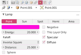
To allow the user to set the color and intensity ("energy") of the point lights we need the corresponding lamp properties panel (we only use color and energy):

This panel is added in the register() function:
    from bl_ui import (
            properties_render,
            properties_material,
            properties_data_lamp,
            )

    ... identical code left out ...

    properties_data_lamp.DATA_PT_lamp.COMPAT_ENGINES.add(CustomRenderEngine.bl_idname)

Code availability

This revision of the code is available from GitHub

Raytracing concepts and code, part 6, specular reflection for lights


This is an article in a multipart series on the concepts of ray tracing. I am not sure where this will lead but I am open to suggestions. We will be creating code that will run inside Blender. Blender has ray tracing renderers of course but that is not the point: by reusing Python libraries and Blender's scene building capabilities we can concentrate on true ray tracing issues like shader models, lighting, etc.
I generally present stuff in a back-to-front manner: first an article with some (well commented) code and images of the results, then one or more articles discussing the concepts. The idea is that this encourages you to experiment and have a look at the code yourself before being introduced to theory. How well this works out we will see :-)

So far the series consists of the several articles labeled ray tracing concepts
Until now the reflections have been a bit dull because our shader model only takes into account the diffuse reflectance, so lets take a look at how we can add specular reflectance to our shader.
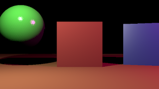
The effect we want to achieve is illustrated in the two images below where the green sphere on the right had some specular reflectance. Because of this it shows highlights for the two points lamps that are present in the scene.


The icosphere shows faceting because we did not yet anything to implement smooth shading (i.e. interpolating the normals across a face) but with added some smooth subdivisions to show off the high lights a bit better.
In the image below we see that we also look at the hardness of the specular reflections in our shader model, with a high value of 400 giving much tighter highlights than the default hardness of 50.


In both images the red cube has no specular intensity and the blue one has a specular intensity of .15 and a hardness of 50.

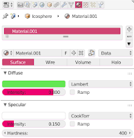
Specular color, specular intensity and hardness are properties of a material so we have also exposed the relevant panel to our custom renderer so that the user can set these values.

Code

The code changes needed in the inner shading loop of our ray tracer are limited:
if hit:
 diffuse_color = Vector((0.8, 0.8, 0.8))
 specular_color = Vector((0.2, 0.2, 0.2))
 mat_slots = ob.material_slots
 hardness = 0
 if len(mat_slots):
  diffuse_color = mat_slots[0].material.diffuse_color \
                    * mat_slots[0].material.diffuse_intensity
  specular_color = mat_slots[0].material.specular_color \
                    * mat_slots[0].material.specular_intensity
  hardness = mat_slots[0].material.specular_hardness

  ... identical code left out ...
  
  if not lhit:
   illumination = light * normal.dot(light_dir)/light_dist
   color += np.array(diffuse_color) * illumination
   if hardness > 0:  # phong reflection model
    half = (light_dir - dir).normalized()
    reflection = light * half.dot(normal) ** hardness
    color += np.array(specular_color) * reflection
We set reasonable defaults (line 2 - 5), override those defaults if we have a material on this object (line 6 - 11) and then, if we are not in the shadow, calculate the diffuse component of the lighting as before (line 16 - 17) and the finally add a specular component (line 18 - 21)

For the specular component we use the Phong model (or actually the Blinn-Phong model). This means we look at the angle between the normal (shown in light blue in the image below) and the half way vector (in dark blue). The smaller the angle the tighter the highlight. The tightness is controlled by the hardness: we raise the cosine of the angle (which is what the dot product is that we compute in line 20) to the power of this hardness. Note that the half way vector is the normalized vector that points exactly in between the direction of the light and the camera as seen from the point being shaded. That is why we have a minus sign rather than a plus sign in line 19 because dir in our code points from the camera towards the point being shaded.

Code availability

The code is available on GitHub.

Raytracing concepts and code, part 5, diffuse color


This is an article in a multipart series on the concepts of ray tracing. I am not sure where this will lead but I am open to suggestions. We will be creating code that will run inside Blender. Blender has ray tracing renderers of course but that is not the point: by reusing Python libraries and Blender's scene building capabilities we can concentrate on true ray tracing issues like shader models, lighting, etc.
I generally present stuff in a back-to-front manner: first an article with some (well commented) code and images of the results, then one or more articles discussing the concepts. The idea is that this encourages you to experiment and have a look at the code yourself before being introduced to theory. How well this works out we will see :-)

So far the series consists of the several articles labeled ray tracing concepts

Our rendered scene so far mainly consists of fifty shades of gray and that might be exciting enough for some but it would be better if we could spice it up with some color.

For this we will use the diffuse color of the first material slot of an object (if any). The code so far needs very little change to make this happen:
            # the default background is black for now
            color = np.zeros(3)
            if hit:
                # the get the diffuse color of the object we hit
                diffuse_color = Vector((0.8, 0.8, 0.8))
                mat_slots = ob.material_slots
                if len(mat_slots):
                    diffuse_color = mat_slots[0].material.diffuse_color
                        
                color = np.zeros(3)
                light = np.ones(3) * intensity  # light color is white
                for lamp in lamps:
                    # for every lamp determine the direction and distance
                    light_vec = lamp.location - loc
                    light_dist = light_vec.length_squared
                    light_dir = light_vec.normalized()
                    
                    # cast a ray in the direction of the light starting
                    # at the original hit location
                    lhit, lloc, lnormal, lindex, lob, lmat = scene.ray_cast(loc+light_dir*eps, light_dir)
                    
                    # if we hit something we are in the shadow of the light
                    if not lhit:
                        # otherwise we add the distance attenuated intensity
                        # we calculate diffuse reflectance with a pure 
                        # lambertian model
                        # https://en.wikipedia.org/wiki/Lambertian_reflectance
                        color += diffuse_color * intensity * normal.dot(light_dir)/light_dist
            buf[y,x,0:3] = color
In lines 5-8 we check if there is at least one material slot on the object we hit and get its diffuse color. If there is no associated material we keep a default light grey color.
This diffuse color is what we use in line 28 if we are not in the shadow.

Code availability

The code is available on GitHub.

Raytracing: concepts and code, part 4, the active camera


This is an article in a multipart series on the concepts of ray tracing. I am not sure where this will lead but I am open to suggestions. We will be creating code that will run inside Blender. Blender has ray tracing renderers of course but that is not the point: by reusing Python libraries and Blender's scene building capabilities we can concentrate on true ray tracing issues like shader models, lighting, etc.
I generally present stuff in a back-to-front manner: first an article with some (well commented) code and images of the results, then one or more articles discussing the concepts. The idea is that this encourages you to experiment and have a look at the code yourself before being introduced to theory. How well this works out we will see :-)

So far the series consists of the several articles labeled ray tracing concepts

In a further bit of code cleanup we'd like to get rid of the hardcoded camera position and look at direction by using the location of the active camera in the scene together with its rotation.
Fortunately very little code has to change to make this happen in our render method:

    # the location and orientation of the active camera
    origin = scene.camera.location
    rotation = scene.camera.rotation_euler
Using the rotation we can first create the camera ray as if it originated in the default -Z direction and then simply rotate it using the camera location:
    aspectratio = height/width
    # loop over all pixels once (no multisampling)
    for y in range(height):
        yscreen = ((y-(height/2))/height) * aspectratio
        for x in range(width):
            xscreen = (x-(width/2))/width
            # align the look_at direction
            dir = Vector((xscreen, yscreen, -1))
            dir.rotate(rotation)
Later we might even adapt this code to take into account the field of vision, but for now at least we can position and aim the active camera in the scene any way we like.

Code availability

The code is available on GitHub.

Raytracing: concepts and code, part 3, a render engine


This is an article in a multipart series on the concepts of ray tracing. I am not sure where this will lead but I am open to suggestions. We will be creating code that will run inside Blender. Blender has ray tracing renderers of course but that is not the point: by reusing Python libraries and Blender's scene building capabilities we can concentrate on true ray tracing issues like shader models, lighting, etc.
I generally present stuff in a back-to-front manner: first an article with some (well commented) code and images of the results, then one or more articles discussing the concepts. The idea is that this encourages you to experiment and have a look at the code yourself before being introduced to theory. How well this works out we will see :-)

So far the series consists of the several articles labeled ray tracing concepts

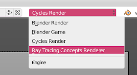
The code presented in the first article of this series was a bit of a hack: running from the text editor and lots of built-in assumptions is not the way to go so lets refactor this in a proper render engine that will be available alongside Blender's built-in renderers:

A RenderEngine

All we really have to do is to derive a class from Blender's RenderEngine class and register it.The class should provide a single method render() that takes a Scene parameter and returns a buffer with RGBA pixel values.
class CustomRenderEngine(bpy.types.RenderEngine):
    bl_idname = "ray_tracer"
    bl_label = "Ray Tracing Concepts Renderer"
    bl_use_preview = True

    def render(self, scene):
        scale = scene.render.resolution_percentage / 100.0
        self.size_x = int(scene.render.resolution_x * scale)
        self.size_y = int(scene.render.resolution_y * scale)

        if self.is_preview:  # we might differentiate later
            pass             # for now ignore completely
        else:
            self.render_scene(scene)

    def render_scene(self, scene):
        buf = ray_trace(scene, self.size_x, self.size_y)
        buf.shape = -1,4

        # Here we write the pixel values to the RenderResult
        result = self.begin_result(0, 0, self.size_x, self.size_y)
        layer = result.layers[0].passes["Combined"]
        layer.rect = buf.tolist()
        self.end_result(result)

Option panels

For a custom render engine all panels in the render and material options will be hidden by default. This makes sense because not all render engines use the same options. We are interested in just the dimensions of the image we have to render and the diffuse color of any material so we explicitly add our render engine to the list of COMPAT_ENGINES in each of those panels, along with the basic render buttons and material slot list.
def register():
    bpy.utils.register_module(__name__)
    from bl_ui import (
            properties_render,
            properties_material,
            )
    properties_render.RENDER_PT_render.COMPAT_ENGINES.add(CustomRenderEngine.bl_idname)
    properties_render.RENDER_PT_dimensions.COMPAT_ENGINES.add(CustomRenderEngine.bl_idname)
    properties_material.MATERIAL_PT_context_material.COMPAT_ENGINES.add(CustomRenderEngine.bl_idname)
    properties_material.MATERIAL_PT_diffuse.COMPAT_ENGINES.add(CustomRenderEngine.bl_idname)

def unregister():
    bpy.utils.unregister_module(__name__)
    from bl_ui import (
            properties_render,
            properties_material,
            )
    properties_render.RENDER_PT_render.COMPAT_ENGINES.remove(CustomRenderEngine.bl_idname)
    properties_render.RENDER_PT_dimensions.COMPAT_ENGINES.remove(CustomRenderEngine.bl_idname)
    properties_material.MATERIAL_PT_context_material.COMPAT_ENGINES.remove(CustomRenderEngine.bl_idname)
    properties_material.MATERIAL_PT_diffuse.COMPAT_ENGINES.remove(CustomRenderEngine.bl_idname)

reusing the ray tracing code

Our previous ray tracing code is adapted to use the height and width arguments instead of arbitrary constants:
def ray_trace(scene, width, height):     

    lamps = [ob for ob in scene.objects if ob.type == 'LAMP']

    intensity = 10  # intensity for all lamps
    eps = 1e-5      # small offset to prevent self intersection for secondary rays

    # create a buffer to store the calculated intensities
    buf = np.ones(width*height*4)
    buf.shape = height,width,4

    # the location of our virtual camera (we do NOT use any camera that might be present)
    origin = (8,0,0)

    aspectratio = height/width
    # loop over all pixels once (no multisampling)
    for y in range(height):
        yscreen = ((y-(height/2))/height) * aspectratio
        for x in range(width):
            xscreen = (x-(width/2))/width
            # get the direction. camera points in -x direction, FOV = approx asin(1/8) = 7 degrees
            dir = (-1, xscreen, yscreen)
            
            # cast a ray into the scene
            
            ... indentical code omitted ...

    return buf

Code availability

The code is available on GitHub. Remember that any test scene should be visible from an virtual camera located at (8,0,0) pointing in the -x direction. The actual camera is ignored for now.

Raytracing: concepts and code, part 2, from rays to pixels


This is an article in a multipart series on the concepts of ray tracing. I am not sure where this will lead but I am open to suggestions. We will be creating code that will run inside Blender. Blender has ray tracing renderers of course but that is not the point: by reusing Python libraries and Blender's scene building capabilities we can concentrate on true ray tracing issues like shader models, lighting, etc.
I generally present stuff in a back-to-front manner: first an article with some (well commented) code and images of the results, then one or more articles discussing the concepts. The idea is that this encourages you to experiment and have a look at the code yourself before being introduced to theory. How well this works out we will see :-)

So far the series consists of the several articles labeled ray tracing concepts

In the first article I presented some code to implement a very basic raytracer. I chose Blender as a platform for several reasons: it has everything to create a scene with objects so we don't have to mess with implementing geometry and the functions to calculate intersections ourselves. It also provides us with the Image class that lets us store the image that we create pixel by pixel when raytracing. Finally it also comes with powerful libraries of math and vector functions, saving us the drudgery of implementing this ourselves. All of this allows us to focus on the raytracing proper.

What is ray tracing?

When ray tracing we divide the image we are creating into pixels and shoot a ray from a point in front of this image (the camera location) into the scene. The first step is then to determine whether this ray hits any object in the scene. If not we give our pixel the background color but if we do hit an object we color this picture with a different color that is dependent on the material properties of the object and any light that reaches that point.

So if we have calculated the location where our first ray (or camera ray, red in the illustration) hits the closest bit of geometry, the next step is to determine how much light reaches that point and combine this with the material information of the object.

There are many ways to approach this and in our first implementation we cast rays from this point in the direction of any lamp in the scene. These rays are often called shadow rays (green in the illustration) because if we hit something that means that an object blocks the light from this lamp and that the point we are shading lies in the shadow of the lamp. If we are not in the shadow we can calculate the light intensity due to this lamp by taking its original intensity and dividing it by the squared distance between our point and the lamp.

Once we have calculated the intensity we can use it to determine the diffuse reflectance. Diffuse reflectance causes light to be scattered in all directions. The exact behavior will be determined by the microstructure of the surface and there are different models to approximate this.

To start we will use the so called Lambert model. In a nutshell this model assumes that incident light is uniformly scattered in all directions which means that if a surface is facing a light it will look bright and this brightness will diminish if the direction of the surface normal diverges from this direction. The brightness we observe is therefore not dependant on the camera orientation but just on the local orientation of the geometry. Different models exist that take into account roughness and anisotropy but that is something for later.

Review: CinemaColour For Blender

Recently I was offered a change to look at CinemaColour For Blender by FishCake.


CinemaColour offers a large collection of professional color management looks (LUTs) to use with Blender's built-in Filmic color management. Check out the artist's website for some great examples. It comes in the form of an add-on that installs over a hundred looks and also offers a convenient way to browse and select the looks that are available. In this short article I'll have a good look at my experiences with the add-on and the looks it offers.

Filmic color management

Since well over a year Blender has incorporated Roy Sobotka's Filmic color management solution and everybody, really everybody, has been very enthusiastic about it ever since. This enthusiasm is well deserved because when using Filmic your renders may almost immediately gain a lot of realism, mainly by mapping the wide range of light intensities in your scene to the limited range of intensities your monitor can handle in a much better way than before. No more blown out highlights or loss in details in the deep shadows!

Looks

Filmic uses lookup tables (LUTs) to convert these intensities and by selecting different look up tables you can create different looks: not only can you choose these looks to present you with more or less contrast in your renders but because these lookups are done independently for all color channels you can use looks that add a color tone to your render. These tones can greatly influence the feel of your scene and because this mapping is done after the result is rendered and composited, it is very easy to experiment with the overall look.

CinemaColour for Blender

Now creating professional looks and making them available for use in Blender is a real craft and that is where CinemaColour comes in. The add-on installs over a hundred different looks and panel in the Scene options where you can easily browse through the list of choices and apply them to your scene. The available looks are grouped in several collections and each look has a name that hints at major blockbuster films that feature a similar look. The available looks range from subtle contrasts to moody color settings and everything in between. Some examples are shown below:

Look: CS ST Y L 3
Look: B2 Gangster
Look: B2 Sniper Alt
Look: B2 The Phantom Alt
Look: B2 Wade Pool
Look: CC Crush
Look: CM Ice
Note that we did not have to render our scene again to generate these looks, so generating these examples after render the scene a single time only took seconds.

Conclusion

A great set of professional looks done by someone who clearly knows their color management. The selection of the provided looks is also intuitive and every artist that is serious about the overall look and feel of their renders should check this out. CinemaColour is available on BlenderMarket.


Raytracing: concepts and code, part 1, first code steps


This is an article in a multipart series on the concepts of ray tracing. I am not sure where this will lead but I am open to suggestions. We will be creating code that will run inside Blender. Blender has ray tracing renderers of course but that is not the point: by reusing Python libraries and Blender's scene building capabilities we can concentrate on true ray tracing issues like shader models, lighting, etc.
I generally present stuff in a back-to-front manner: first an article with some (well commented) code and images of the results, then one or more articles discussing the concepts. The idea is that this encourages you to experiment and have a look at the code yourself before being introduced to theory. How well this works out we will see :-)

So far the series consists of the several articles labeled ray tracing concepts

In this article I will show how to implement a minimal raytracer inside Blender. Of course Blender has its own very capable renderers, like Cycles, but point is to illustrate some ray tracing concepts without being bogged down with tons of code that have nothing to do with ray tracing per se.

By using Blender's built-in data structures like a Scene and an Image and built-in methods like ray_cast() we don't have to implement difficult algorithms and data structure like ray/mesh intersection and BVH-trees for example, but we can concentrate on things like primary and secondary rays, shadows, shading models etc. etc.

The scene

The scene we will be working with at first looks like this:

Nothing more than a plane, a couple of cubes and an icosphere. Plus two point lights to illuminate the scene (not visible in this screenshot).

In rendermode the scene looks like this:

Note that we didn't assign any materials so everything is shaded with a default shader.

Our result


Now the result of the minimal raytracer shown in the next section looks like this:
There are clear differences of course, and we'll work on them in the future, but the general idea is similar: light areas close to lights and visible shadows. How many lines of code do you think is needed for this?

The code


The code to implement this is surprisingly compact (and more than half of it is comments):
import bpy
import numpy as np

scene = bpy.context.scene

lamps = [ob for ob in scene.objects if ob.type == 'LAMP']

intensity = 10  # intensity for all lamps
eps = 1e-5      # small offset to prevent self intersection for secondary rays

# this image must be created already and be 1024x1024 RGBA
output = bpy.data.images['Test']

# create a buffer to store the calculated intensities
buf = np.ones(1024*1024*4)
buf.shape = 1024,1024,4

# the location of our virtual camera
# (we do NOT use any camera that might be present)
origin = (8,0,0)

# loop over all pixels once (no multisampling)
for y in range(1024):
    for x in range(1024):
        # get the direction.
        # camera points in -x direction, FOV = 90 degrees
        dir = (-1, (x-512)/1024, (y-512)/1024)
        
        # cast a ray into the scene
        hit, loc, normal, index, ob, mat = scene.ray_cast(origin, dir)
        
        # the default background is black for now
        color = np.zeros(3)
        if hit:
            color = np.zeros(3)
            light = np.ones(3) * intensity  # light color is white
            for lamp in lamps:
                # for every lamp determine the direction and distance
                light_vec = lamp.location - loc
                light_dist = light_vec.length_squared
                light_dir = light_vec.normalized()
                
                # cast a ray in the direction of the light starting
                # at the original hit location
                lhit, lloc, lnormal, lindex, lob, lmat = scene.ray_cast(loc+light_dir*eps, light_dir)
                
                # if we hit something we are in the shadow of the light
                if not lhit:
                    # otherwise we add the distance attenuated intensity
                    # we calculate diffuse reflectance with a pure 
                    # lambertian model
                    # https://en.wikipedia.org/wiki/Lambertian_reflectance
                    color += intensity * normal.dot(light_dir)/light_dist
        buf[y,x,0:3] = color

# pixels is a flat array RGBARGGBRGBA.... 
# assign to a single item inside pixels is prohibitively slow but
# assigning something that implements Python's buffer protocol is
# fast. So assiging a (flattened) 1024x1024x4 numpy array is fast
output.pixels = buf.flatten()
I have added quite some comment in the code itself and will elaborate on it some more in future articles. For now the code is given as is. You can experiment with it if you like but you do not have to type it in nor create a Scene that meets all the assumptions in the code, you can download a .blend file that contains the code if you like.

Code availability

The files are available from my GitHub repository:

The code itself

A .blend file with a full scene and the code embedded as a text file (click Run Script inside the text editor  to run it)