Starfield example
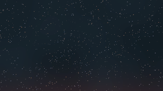
The image below is a still from a short animation.
(It is pretty dark, for cinematic effects you probably would choose a far brighter setup)
The stars are generated with the starfield shader and their distribution is controlled by a noise texture. The faint green glow of stellar dust and the faint orange color on the horizon are generated with a separate noise and gradient texture respectively. (example node setup at the end)
The animation features additional twinkling that is not visible in the still image. This is effected by blending time animated 4d simplex noise.
(In the animation the contrast/lightness was autocorrected for a better view)
The code
The code below contains two functions: one that calculates a probability dependent voronoi distribution and the shader itself. The code is pretty straight forward but note that theFalloff value should not be set too high to prevent artifacts in the star shapes when seen in close-up. (These are due to the fact that we divide space in cells and the fact that we only considered the nearest neighboring cells for our voronoi distribution. Taking into account further neighbors would solve this but impact the performance of the shader in a rather drastic manner).The outputs of the shader consist of a color and a factor. The color is the emmisive power in W/m2. This could be used as an input to an emmision closure but in fact it might be simpler just to normalize this and use it as a color directly (as is done in all examples). The factor is just a value which is 1.0 for the center of the stars aand decreases exponentially when further away.
point voronoi3dp(point p, float density, output float d2)
{
 int xx, yy, zz, xi, yi, zi;

 xi = (int)floor(p[0]);
 yi = (int)floor(p[1]);
 zi = (int)floor(p[2]);

 float dbest = 1e10;
 point pbest = 1e10;
 vector dz = vector(7,111,19);
 for (xx = xi - 1; xx <= xi + 1; xx++) {
  for (yy = yi - 1; yy <= yi + 1; yy++) {
   for (zz = zi - 1; zz <= zi + 1; zz++) {
    vector ip = vector(xx, yy, zz);
    if(cellnoise(ip)< density){
     point  vp = ip + cellnoise(ip+dz);
     vector dp = p-vp;
     float  d  = dot(dp,dp);
     if (d < dbest) {
      dbest = d;
      pbest = vp;
     }
    }
   }
  }
 }
 d2=dbest;
 return pbest;
}

shader stars(
 point Pos = P,
 float Stardensity = 0.001,
 float Scale = 1000.0,
 float Falloff = 10,

 output color col = 0.0,
 output float fac = 0.0
){
 point p = Pos * Scale;

 float d;
 voronoi3dp(p,Stardensity,d);
 fac = exp(-d*Falloff);
 if(d<100 br="">  col = blackbody(3500.0+6000.0*cellnoise(p+vector(17,17,17)));
 }
}
Example node setup
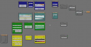
The node setup used to generate both the still image and the animation is shown below. It's fairly large but not really complicated.
(click to enlarge)
Each texture contribution is ordered in a horizontal row of nodes. From top to bottom: the starfield (dark blue, note the normalization of the color), the twinkling (light blue), the dust (green) and the horizon glow (yellow). The glare was added in the compositor along with some contrast enhancement (for the video sample I added extra contrast enhancement in an external program). An example .blend file bundled with the stars.osl script and the simplexnoise.osl script is available as a .zip file on GitHub. (click
View Raw button to download) 