Small Blender Things: open shading language

Showing posts with label open shading language. Show all posts

Open Shading Language for Blender on BlenderMarket

The last couple of weeks I have been working to create a distribution channel for my Blender related e-books that is better suited to the intended audience. And what better distribution channel than BlenderMarket! With special thanks to Jonathan and Matthew I am happy to announce the first result is there:
Open Shading Language for Blender is now also available on BlenderMarket:

(click on the image to go to the shop where you can read the description and download a sample chapter)

Noise experiment with Open Shading Language

I am still looking for good procedural noise to be used as the basis for bark materials. Such noise would need some anisotropy because the cracks in bark are almast always oriented: either along the direction of the trunk or perpendicular to it, depending on the stretching characteristics during growth. Now you could scale for example Perlin noise or use Gabor noise (the latter is available in OSL as well, check for example this article), but we could also create it from scratch.

Theory

In the shader we randomly distribute a number of line segments through space and calculate the distance to these line segments. If we are close enough to a segment we add a value to our sum and in the end the value for a pixel is the sum of all these contributions. Now the essence is in the distribution of those line segments because we do not only control their length but also how far they may deviate from a preferred direction.
The code for the shader itself is quite simple (I have omitted all auxiliary functions):

shader dtnoise(
 point  Pos = P,            // texture position and scale
 float  Scale = 1,
 
 int    Np = 15,            // number of ticks (impulse) per cell
 
 int    Seed = 42,          // random seed
 
 float  Radius = 0.3,       // distance to impulse that will add to result
 float  Size = 0.7,         // length of an impulse
 vector Dir = vector(1,0,0),// direction of anisotropy
 float  Theta = M_PI/2,     // cone (half)angle. The default = 90% which means no anisotropy
 
 float  Step = 0.3,         // cutoff value for Fac output
 float  Gain = 0.3,         // brightness of the result
 
 output float Sum = 0,      // the sum of all the tick values
 output float Fac = 0       // the 
){
 point p = Pos * Scale;
 point f = floor(p);

 vector an= normalize(Dir);
 vector r = vector(an[2],an[1],an[0]); //no need to norm again
 vector uv = cross(an,r);
 vector vv = cross(an,u);

 
 int xx,yy,zz, np;
 
 int nn[3];
 
 for( xx=-1; xx<=1; xx++){
  for( yy=-1; yy<=1; yy++){
   for( zz=-1; zz<=1; zz++){
    point ff = f + vector(xx,yy,zz);
    int s=Seed;
    
    nn[0] = int(ff[0]);
    nn[1] = int(ff[1]);
    nn[2] = int(ff[2]);
    
    for( np=0; np < Np; np++){
     vector pd1 = noise("cell",ff,s);
     vector pd2 = randomcone(uv, vv, an, Theta, nn, s+1);
    
     point p1 = ff + pd1;
     point p2 = p1 + Size * pd2;
    
     float d = distance(p1,p2,p);     
     Sum += (1 - smoothstep(0, Radius, d));
     
     s+=3;
    }
   }
  }
 }
 
 Sum *= Gain;
 Fac = smoothstep(0, Step, Sum);
}

The essence is in line 44 and 45: here we pick a random point and another point along a random direction, where this random direction is restricted to a cone whose narrowness we can control with the Theta parameter. Those two points make up the start and end points of a line segment and if the distance to this line segment is small enough we a a value. (make sure that the sum of Size and Length < 1 to prevent artifacts.

Samples

With few points per cell the anisotropy is very clear (left: Theta = 0.05, right Theta = 1.51 (approx. 90 degrees):

Adding points increases the complexity of the noise (we reduced the gain, the number of points is 40):

If we compare our noise to gabor and perlin noise (each thresholded and suitably scaled in a preferred direction) we see that the patterns are similar but each with its own character.

How useful this all is, it up to you of course :-) It is nice to have a different procedural noise in your toolbox but on the other hand, it ties you to OSL (i.e. you can't use it on the GPU) and it is relatively slow.

Code availability

As usual the full code is available on GitHub.

Mmmm, maybe this advertising widget below is a bit over sized. Still, if you would like to learn some more about Open Shading Language for Blender, you might check it out.

Voronoi noise with cyclic metrics, an experiment

While working on adding more functionality on voronoi nodes in OSL I was wondering if we could vary the metric in some interesting way. The result of one of those experiments is shown below:

The noodle used to generate this image looks like this:

Note the number 7 in de metric drop down.

Observations

The pattern looks decidedly different from other cell like patterns and depending on the value of E can be made to look like anything from x-ray diffraction pattern(? at E=28) to stylized models of atoms (E=2.6):

The code for this metric(*) is this:
length(d) + (1 + sin(e * length(d)))/2;
i.e. we basically add a sine component to the distance. If E is zero this metric reduces to a plain distance metric. (*) Note that this isn't a true metric in the mathematical sense as it does not satisfy the triangle inequality.

Code

The code is a minor adaptation of my previous script and is available on GitHub.

If you would like to know more about programming OSL you might be interested in my book "Open Shading Language for Blender". More on the availability of this book and a sample can be found on this page.

Fast Voronoi F2F1 in Blender Cycles on GPU and CPU

The voronoi noise texture in Blender Cyles is rather limited: it is only based on the distance to the nearest point while many interesting patterns need the distance to the next nearest points as well (or the difference F2 - F1). Also there is no way to vary the distance metric, everything is based on the distances squared while for example so called manhattan metrics yield squarish patterns that can be quite useful.

I did submit the path for review just now, if you're interested you can follow its fate here.

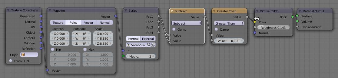
All of this can be overcome by using Open Shading Language, but the Cycles OSL implementation is limited to the CPU and cannot benefit from a much faster GPU. I therefore decided to try and implement it in the Blender source code and that went rather well (but see my rants below):

As you can see I added a second value output to the Voronoi node that yields the distance to the next nearest neighbour and added a dropdown to select the distance metric. Currently I have implemented the distance, distance squared (the default), manhattan and chebychev metrics, I might add the generalized minkowsky metric as well. The images show the F2 - F1 noise for the distance squared and manhattan metrics respectively:

The code works on GPU and on CPU but I only tested it on 64bits Linux (Ubuntu 15.04 to be precise) although there is no reason to believe it will work differently on antoher OS.

Can I haz codez?

The diff to the Blender source code as of 8/8/2015 is for the time being available via DropBox. If there is enough positive feedback I will try to get the patch accepted for inclusion in the source code. Note that the diff shows also some changes to files that have nothing to do with the node itself, notably device_cuda.cpp, which i need to tweak because although I have a GTX970 (= SM_52 capable) card, I didn't upgrade my cuda drivers so i needed to hack the source to restrict the cuda compiler to sm_50. This is irrelevant to the patch itself.

Some remarks about the code: coding this was not all pleasure and that is an understatement. No less than 8 files needed to be changed to alter a single node type. That isn't a bad thing in itself but there is duplicated code, a lot of redundant constants defined in different places and I could find no decent documentation on the stack based virtual machine (svm) that is used by Cycles. It took me way longer to fathom the ins and outs of the code than it took to write the code itself and I am still not 100% certain that I did not miss something. Blender is a wonderful piece of software but it certainly would benefit from a set of decent architecture docs :-)

Renderman for Blender vs. OSL

Everybody is thrilled because of Pixar's decision to offer a version of Renderman that is free for non-commercial use, and rightly so because it will enable a lot of people to get acquainted with this industry standard.
Even better is the support by Pixar for a tight integration of Renderman with Blender, in the form of an open source add-on. This add-on may not be production quality yet, but once you have installed Renderman it works out of the box:

Open Shading Language

From my point of view Renderman is extra interesting because it supports shaders written in Open Shading Language (OSL) which means that we should be able to port OSL shaders written for Cycles to Renderman. In the image of Susanne the patterning on her head was actually done by plugging in this simple OSL shader:

shader marble (color Cin = .5,
               float freq = 1.0,
               output color result = 0)
{
    float sum = 0;
    float freqVal = freq;

    point Pshad = transform ("object", P);
    for (int i = 0; i < 6; i++) 
    {
        sum = sum + 1/freqVal * abs(.5 - noise( 4 * freqVal * Pshad)) ;
        freqVal = 2 * freqVal;
    }
    result = Cin * sum;
}

Workflow

There are a couple of restrictions and quirks so let me walk you through the steps I took to get this shader running.

Compile the shader

Renderman will not compile OSL shaders automatically for you like Cycles does, so you will have to do that yourself. If you do not have the oslc compiler installed separately the easiest way to do this is to create a Cycles material first that contains a Script node. When you refer this Script node to an external .osl file it gets compiled immediately to an .oso file and this .oso file can be used as is by Renderman.

Link it to the diffuse color

First select a PxrOSL pattern by clicking the dot next to the baseColor, and then type in the full path to the shader, but without the .oso externsion! (circled in red)

You will notice in the node editor that a PxrOSL node is wired up to the PxrDisney shader.

At this point you can render your scene.

Quirks

If you look closely at the PxrOSL node and at the code for the shader you see that the input and output sockets correspond just partially to the input and output parameters of the shader. Indeed, all input parameters are completely ignored and there is an extra float output socket called result1. The types and names of the input and output sockets are it seems defined in the file /opt/pixar/RenderManProServer-20.0/lib/RIS/pattern/Args/PxrOSL.args and are the same for all OSL shaders. So as far as I understand it, you can use different shaders but they all should use the same names for their input and output sockets (I think this is in line with other Renderman patterns). For this example it meant that I had to rename the output color from Cout to result to get it working (otherwise you get a rendertime error complaining it cannot link to the result socket). Maybe I am looking at it from the wrong perspective as I know next to nothing about Renderman, It is workable of course, just define enough suitable input and output parameters and use those predefined names in your shader but it feels a bit restrictive. Anyway, it is a very promising step. I am studying the add-on to see if I can tweak the OSL node part and maybe help out the original author.

Voronoi playtime, redux

In a previous article I showed how some hidden functionality in Blender's distributed OSL headers could be used to create all sorts of Voronoi/Worley noise. At that point I left out the choice of distance metric because there wasn't a nice way to implement choices in OSL.

There still isn't but prompted by a question I decided to implement it in an ugly way; after all, if it works that is all that matters :-). All the necessary code to implement different distance metrics is already in node_texture.h but for some reason it was commented out. I therefore lifted the necessary part from this file and combined it with a a small shader that lets you choose the distance metric with an integer. An example for the Manhattan metric is shown below.

Node setup and code availability

The node setup used to generate the image above looks like this:

The code for the shader is available on GitHub. The node it generates may look a bit different than in the noodle shown here because I added an exponent input E that can be used for the generalized Minkovsky metric (metric == 6).

Greebles in OSL

The shader that is presented here basically takes as input a set of uv coordinates and produces a set of rectangles, each with their own uv coordinates. These rectangles are randomly distributed and rotated and do not necessarily cover everything: the fac output signals whether there is a rectangle or not.

With this set-up you can for instance cover a surface with random hull plates or similar:

The noodle used to produce the image looks like this:

There are two OSL shaders in this noodle: the first one on the left is called Greebles and is the one that divides up the coordinate space, the second one is called Rivets and is part of the green Rivets material layout. That last one simply distributes small circles around the edges of a rectangle.

Both shaders are available on GitHub, Greebles here, and Rivets here.

Strips OSL Shader: subdivide a uv map into strips and slots

In an ongoing effort to search for methods that can be used to generate bark textures I devised this simple OSL shader: it takes a uv-map (for example one that is wrapped around a cylinder representing a branch ans subdivides this in to strips. These strips are then subdivided into slots and each of these slots is given its own uv map and a random value.

This simple setup makes it possible for example to combine two tileable images in a manner that resembles bark an knots or cracks in that bark. The example below shows the result with two simple black and white images, mapped to a plane a a cylinder:

The underlying slots look like this:

Example node setup and code availability

The example node setup used to create both of the images above looks like this (click to enlarge):

The shader is availble on GitHub along with two sample textures: 1, 2.
The code should contain enough comments to get you going, but just tweaking the input parameters based on the example noodle should get you a long way.

Chaos mosaic with OSL

Chaos mosaic is a technique tht can be used to reduce the repetative appearance of tilebale images. An example is shown below. The upper right plane shows visible repetition artifacts that are not apparent in the lower left plane.

(I used a 700x700 tileable texture from CGtextures.com (Gravel0170_3_S.jpg) repeated four times in each direction on the upper right plane, and the same image with the chaosmosaic shader on the lower left plane)

Shader code

The shader code to implement this is very short:

shader chaosmosaic(
  point Pos=P,
  string Image="",
  int M=10,
  
  output color Color=0
){
  float x,y;

  x=mod(Pos[0],1);
  y=mod(Pos[1],1);
  
  float xi=floor(x*M);
  float yi=floor(y*M);
  
  // mapping here
  float xp=noise("cell",Pos,xi*M+yi);
  float yp=noise("cell",Pos,xi*M+yi+M*M);
  
  float xoffset = mod(mod(x,1.0/M)+xp,1);
  float yoffset = mod(mod(y,1.0/M)+yp,1);
  Color = texture(Image,xoffset,yoffset);
}

In the code above M is the number of squares in each direction in our uv map. We use it to calculate two indices (xi, and yi) that are subsequently used pick a random position in the texture (xp,yp). The pixel from the texture is then selected according to the relative offset in the small square inside the uv map (xoffset, yoffset). The original algorithm also uses a blending function between adjacent tiles form the textures but that will blur the image. In this case we didn't implement that because from far enough away the small tile edges aren't noticable but the large scale repetion has gone away so with very little code we already have a better result.

Example node setup

The node setup used for the example image (the plane on the lower left) looks like this:

reference

http://en.wikipedia.org/wiki/Texture_synthesis#Chaos_mosaic
http://research.microsoft.com/apps/pubs/?id=69770 (the research paper)

A hexagon shader in OSL, second edition

A while ago I made a simple OSL shader for hexagonal tilings. Prompted by some questions on BlenderArtists I decided to create a more versatile version that retained the color options but added the distance to the closest edge. That feature may help in creating crips edge patterns because the previously availble distance to the closest center creates rounded shapes that might be suitable for bee hives but not for hard edged stuff like floor tiles etc.

The noodle used to create the image is shown below (click to enlarge):

The color code has stayed the same except for the calculation of the distance to the edge. This might be a bit inefficient, but at least it's easy to read.
The additions are shown below, the full code is available on GitHub.

    // distance to nearest edge
    
    float x = mod(Coordinates[0]/3,1.0);
    float y = mod(Coordinates[1]/3,A2);
   
    #define N 18
    vector hc[N] = {
        vector(  0, -A2/3     ,0),
        vector(  0,     0     ,0),
        vector(  0,  A2/3     ,0),
        vector(  0,2*A2/3     ,0),
        vector(  0,  A2       ,0),
        vector(  0,4*A2/3     ,0),

        vector(0.5, -A2/3+A2/6,0),
        vector(0.5,     0+A2/6,0),
        vector(0.5,  A2/3+A2/6,0),
        vector(0.5,2*A2/3+A2/6,0),
        vector(0.5,  A2  +A2/6,0),
        vector(0.5,4*A2/3+A2/6,0),

        vector(1.0, -A2/3     ,0),
        vector(1.0,     0     ,0),
        vector(1.0,  A2/3     ,0),
        vector(1.0,2*A2/3     ,0),
        vector(1.0,  A2       ,0),
        vector(1.0,4*A2/3     ,0)
    };
    
    float d[N], t;
    
    for(int i=0; i < N; i++){
        float dx = x - hc[i][0];
        float dy = y - hc[i][1];
        d[i] = hypot(dx, dy); 
    }
    
    for(int j= N-1; j >= 0; j--){
        for(int i= 0; i < j; i++){
            if(d[i] > d[i+1]){ 
                SWAP(t, d[i], d[i+1]);
            }
        }
    }
    
    Center  = d[0];
    Edge    = d[1] - d[0];
    InEdge  = Edge < Width;

The approach we have taken is very simple: the hc enumerates all nearby hexagon centers. We then calculate all the distances to these points and sort them shortest to longest (yes with a bubble sort: with 18 elements it might just be faster to do it with a more efficient sorting algorithm at the cost of much more complex code so I don't bother).
The Edge is not realy the distance to the closest edge but the difference between the closest center and the next closest. Near the edge these values are more and more the same so Edge will approach zero. For convience we provide a comparison with some threshold also.

Settling of particles in suspension with Blender and OSL

Playing with volumetrics I wanted to approximate the effect of the settling of suspended particles from a fluid, like what happens when you leave a glass of orange juice standing for too long. The idea is that there is some region near the bottom of the glass that has a dense mass of settled particles and that in the beginning the diminishing density towards to surface is not all that visible but get clearer with time.
Of course this could be implemented with math nodes but I find it far simpler to write it all down in OSL and condense the logic in a single script node. The result shown below is admittedly not the animation that will get nominated for the next Academy Award but does show nicely the slow settling I had in mind, including the effect that near the end the fluid seems to clear up quicker:

OSL code and node setup

The node is simple enough:

shader edgedecay(
    point Pos    = P,
    float Edge   = 0.1,
    float Power  = 1,
    float Density= 10,
    float Length = 1 - Edge,
    
    output float Fac=Density
){
    float h = Pos[2];
  
    if(h>Edge){
        float d = (h - Edge)/Length;
        if(Power > 0 && d < 1){
            Fac = Density * ( 1 - pow(d,Power));
        }else{
            Fac = 0;
        }
    }
}

The node setup for the videoclip is:

The Density input was animated from 2.7 to 3.5 in 100 frames, while at the same time the Power input was animated from 1.0 to 0.0.
The following graph shows the plot of the density profile with relevant parameters:

OSL support in mainstream renderers (V-Ray and Renderman)

Things are getting interesting now that more major players start supporting OSL. This week Pixar announced the support for OSL in Renderman and a few months ago Chaosgroup released a version of V-Ray with OSL integration.

Not all integrations are equal, for example the one in Renderman doesn't appear to support closures (bsdf's), but nevertheless, now there is a huge potential to share programmatical patterns and textures between V-Ray, Renderman and Blender. I am quite exited and can't wait to see how this will foster the reuse of shaders across platforms. To illustrate the portability: some of the shaders provided as examples on the V-Ray page work on Blender without a single change, while others need some tweaks, mainly because each renderer provides its own set of closures (for eaxmple, Blender does not have the phong() closure) and more importantly, the output model is not identical: the V-Ray shaders don't provide closure outputs, but simply assign to the Ci variable, something that on Blender has no effect.

A new tree addon, Part IV: volume rendering experiments with OSL

With the new volume shading options offered by Blenders OSL implementation it is tempting to try this on the trees generated by the space tree addon. Without adding any extra geometry or particles apart form a basic ahape a volume shader might give the impression of a much denser crown as shown in the image below:

This effect was achieved by inserting a scaled icosphere that covers about 90% of the crown interior (see below) and adding a volume shader to this icosphere that scatters and absorbs light in a non-uniform manner, i.e. the shader mimics a bunch of small scattered disks, which when seen from the distance add to the illusion of leaves. Note that we cannot do without all the leaves because volume scattering adds no specular reflections as real leaves might do.

Shader code and example node setup

The code for this shader consists of the shader proper, which merely checks which randomly scattered point we are closest to and then calls the indisk function with the position of this closest point and a random direction. indisk checks whether we are inside a disk with its axis in some direction and returns 1 if this is indeed so. Note that the include at the start of the code refers to a file that is distriubted with Blender and contains a number of useful functions, including a number of Voronoi/Worley related ones.

#include "node_texture.h"

int indisk(
  point p,
  point c, float r, float h, vector d
){
  vector v = p - c;
  float a = dot(v,d);
  float lh = abs(length(a * d));
  if(lh > h){ return 0;}
  float lv = length(v);
  float lp = sqrt(lv*lv - lh*lh);
  if(lp > r){ return 0;}
  return 1;
}

vector randomdirection(point p){
  float t = M_2PI*noise("cell",p,1);  
  float u = 2*noise("cell",p,2)-1;  
  float s,c,a;  
  sincos(t,s,c);  
  a = sqrt(1-u*u);  
  float x = a*c;  
  float y = a*s;  
  float z = u;  
  return vector(x,y,z);
}

shader bits(
  point Pos = P,
  float Scale = 1,
  float Size = 1,
  float Height = 0.05,

  output float Fac = 0
){
  point p = Pos * Scale;
  point centers[4];
  float distances[4];
  voronoi(p, "Distance Squared", 0, distances, centers);
  if(indisk(p,centers[0],Size,Height,randomdirection(p))){
    Fac = 1;
  }
}

The node setup to use this shader as seen in the opening image of this article looks like this:

Discussion

Whether using a volume shader this way is really useful remains to be seen: rendering this way is still rather slow. Of course, getting a comparable dense crown with extra particles also slows down rendering: in my tests doubling the number of particles from 1000 to 2000 resulted in a render time that was actually slower than adding the volume shader. In other words, your mileage may vary but it might be worth to experiment.

References

The space tree addon itself is introduced in a few articles on this blog and is available on GitHub. Relevant links are listed below:

OSL Bevel Shader

In a BlenderArtists thread about ambient occlusion shaders the question was asked if OSL's ray tracing capabilities coudl be used to create a bevel shader, i.e. a s shader that mimics rounded edges on sharp meshes by manipulating the normal. I think the answer to this question is 'yes' and in this post I'' show a first implementation (Edit: the previous code did normalize the resulting normal, now it does. You can follow the discussion on this thread)

Sample scene, just a cube and an icosphere with sharp edges and some glossy material.

The effect of the bevel shader with Perturb = 0.1. Subtle but clearly noticable.

Setting Perturb = 1.0 is far less subtle but shows how much roundedness is possible. All images were produced with Divisions = 3, i.e. 27 sample rays (see below).

Code & theory

To simulate rounded edges choose a point a little below the surface and from this point we cast a set of rays that are all a little bit perturbed from the normal. The we determin the normal at these new intersections and average all normals found. This way when we are close to an edge the normals at the intersection with an adjacent face will be blended in. The illustration below shows what I mean:

At the shaded point we have a green surface normal. We descend below the surface along this normal (dashed red line) to the blue point. From this point we shoot rays (red) that are slightly perterbed from the normal. Some will hit the same face (and have the same normal as the shaded point (small blue arrows) some will hit the adjacent face with adifferent normal (small orange arraws). The calculated normal is the average of the normals at the hit points.
Note that this algorithm only works well for convex edges, because with concave edges random faces could be hit instead of the adjacent face if the angle between the faces is too sharp.
The code implementing this algorithm is pretty short:

#define BIG 1e6

shader edge(
  float Delta = 0.01,
  float Perturb = 0.001,
  int Divisions = 2,
  output float Fac = 0,
  output normal Normal = N
){
  vector origin = P-Delta*N;
  float count = 1;
  for(int x=0; x < Divisions; x++){
    for(int y=0; y < Divisions; y++){
      for(int z=0; z < Divisions; z++){
        vector d = noise("perlin",vector(x+0.1,y+0.1,z+0.1));
        vector np = N + Perturb * d;    
        if(trace(origin, np)){
            float hdb = 0;
            normal nb = 0;
            getmessage("trace","hitdist",hdb);
            // versions before 2.69.11 4-Mar-2014 crash on next statement
            getmessage("trace","N",nb);
            Normal -= nb;
            count += 1.0;
        }
      }
    }
  }
  Normal = normalize(Normal/count);
  Fac = count/(1+Divisions * Divisions * Divisions);
}

We choose an origin point a bit below the surface by descending along the normal [line 10], generate perturbed normals [line 15-16], trace these normals [line 16] and if we have a hit we retrieve the normal at the hit point [line 22]. Because we are below the surface/ inside the mesh this normal will point inward so we subtract it from our sum of normals (Normal). Finally we divide the sum of normals by the number of hits [line 30]. Note that we also get the hit distance [line 20] but don't use that value. We could check this againt some limit to reduce artifacts on concave meshes for instance.
The generation of perturbed normals is rather awful: just perturbing it by Perlin noise does not give a very uniform distribution of directions, some Halton or Sobel sequence would probably be better but this will do for now. Also not we add a small value too our noise sampling points to avoid the zeo knots in the Perlin noise.
Also note that I got crashes with Blender's daily build version before March 4 (win-64 version) when using the getmessage() function. This appears to be fixed in the latest builds but be aware.

Example node setup

Note that the node does not take a position or normal as input, it gets those from the global P and N respectively but of course if necessary this can be changed quite easily. The setup shown below is the exact setup used for the example images at the start of the page.

Drawing cubic splines in OSL

Some time ago I wrote about a routine to calculate the closest distance to a quadratic bezier spline and recently I reused this routine again in a slightly optimized form to create wiggles.
Being able to calculate the closest distance to a quadratic spline is useful but I really wanted to use cubic splines because they offer more control, allowing for easier ways to create nice shapes.

update: made the code 10% faster by making it 2D only. The GitHub version relects that change but original code can be used by removing a single macro
Warning; long read ahead :-) The first section describes how to use the shader and where to download the code and is pretty short. The second section dives deep into the code and is definitely not an easy read, sorry for that but fortunately there is no need to go that deep if you know what a cubic spline is and just want to use the code.

The shader

The approach to finding the distance to a cubic spline is the same in principle as for a quadratic spline: find all values for t that satify the relation dB(t)/dt . (B(t) - P) = 0, or in English: those values of t whre the tangent to the spline is perpendicular to the vector pointing to the point being shaded (remember that the dot product of two vectors is zero if they are perpendicular).
For a quadratic bezier curve the equation to solve is cubic and is quite simple but for a cubic bezier curve this is a fifth order equation for which there is no analytical solution. And although cubic splines are used everwhere (for example in fonts) a numerical solution for this problem was surprisingly hard to find.
Fortunately after some serious searching the Graphic Gems series of books proved again to be incredible useful, specifically "A Bezier Curve-Based Root-Finder" by Philip J. Schneider.
The original code is in C so it neede quite some work to convert it to OSL. Normally converting C code to OSL is pretty straightforward but this code uses multidimensional arrays and recursion, both unknown to OSL. On the plus side, OSL's native point type and built-in dot() make for a lot less code.

Code availability and node setup

My implementation (with a sample shader in the same file) is available on GitHub. The node setup used to create the heart shape is shown below, it is made of two mirrored splines:

The values for the control points are:P0 = ( 0.5, 0.1, 0.0)
P1 = (-0.5, 0.7, 0.0)
P2 = ( 0.4, 1.2, 0.0)
P3 = ( 0.5, 0.8, 0.0)

Code explanation

I am not going to list all of the code because it's way to long and rather boring but I will tell some more about the FindRoots() which is nontrivial and needed to be reimplemented in a non-recursive form.
The general idea of the shader to cast the fifth order equation whose roots we'd like to find in a form that is itself a bezier curve (I.e. a bernstein polynomial) and exploit the specific properties of a bezier curve to efficiently find the roots.
The mathematical specifics are explained very well in Schneider's article so let us just look at the code:

#define POP wtop+=6;wn--

int FindRoots(point w0[6], float t[5]){
  point w[STACKSIZE];
  int wtop=0;
  int wend=0;
  int wn=0;
  for(int k=0;k<6 br="" k="" w0="" w="" wend="">  wn++;
  int nc=0;
  while(wn>0){
    //printf("[%d]",wn);
    int cc=CrossingCount(w,wtop); // w[:5]
    if(cc==0){
      POP;
      continue;
    }
    if(cc==1){
      if(wn>=MAXDEPTH){
        t[nc++]= (w[wtop][0]+w[wtop+5][0])/2;
        //printf(" MAX ");
        POP;
        continue;
      }
      if(ControlPolygonFlatEnough(w,wtop)){ // w[:5]
        t[nc++]= ComputeXIntercept(w,wtop);
        //printf(" FLAT (%.1f | %.1f)",w[wtop],w[wtop+5]);
        POP;
        continue;
      }
    }
    // not flat or more than one crossing
    DeCasteljau(w,0.5,wtop,wend);  //left=[wend:wend+5], right=[wend+6;wend+11]
    for(int k=0;k<6 br="" k="" w="" wend="" wtop="">    wn++; wend+=6;
  }
  return nc;
}

A fifth order bezier curve has 6 control points and at most 5 roots. The control points are passed as the w0 argument and the t array will receive the root values. The function's return value will be the number of roots found.
The central idea of this algorithm is to find a segment of the curve that crosses the x-axis just once and then determine the intercept, i.e. a root. To achieve this the spline is subdived into to halves, each again a fifth order spline, until such segment contains a single crossing.
Because OSL doesn't support recursion, we have to maintain a stack of control points ourselves and that's where the w array comes in.
Starting with the for-loop in line 8 we transfer the initial set of 6 control points to the stack and adjust wn to reflect that we now have one set on the stack. At this point wtop (the index of the first control point in the topmost set) is 0, and wend (the index of the first free slot in w) is 6. nc holds the number of roots found sofar.
Next we iterate as long as there is a set of control points on the stack (line 11). We caculate how many times the curve defined by this set crosses the x-axis. If there is no crossing there is no root in this curve so we pop the set of the stack and continue.
If there is a single root and we have recursed deep enough we simply approximate the root as lying halfway between the x-coordinates of the first and last control points and pop the set (line 20). If there is room to recurse we check whether the set of control points is "flat enough" (line 25) and if so compute the intercept with the x-axis of the line between the first and last control point. We store this root and pop the set of control points (see Schneider's article or the original source code to see what is meant by "flat enough").
If the control points are not "flat enough" or we have more than one root in this curve, we split the curve in two using DeCasteljau's method (line 33). The function will produce two sets of six control points at position wend in the w array. The save space we copy the second set to top of the stack (because the control points for the original curve are no longer needed), which means we only have to increase the stacksize wn by one.
Finally, if we run out of the while-loop we simply return the number of roots found.

Speed

Now you might think that all this recursion and the numerous calculations would be very slow but you will be surprised. The function seldom needs to recurse very deep because the accuracy used to determine if a curve is "flat enough" need not be that good (we can't see differences much less than a pixel). On my machine this means that I can tweak the node setup for the example image at interactive speeds if I set the number of preview samples to 1.
There is however plenty of room for optimization, especially in areas were we do calculations with 3D points. If we only want to work in 2D we might save up to 30% on unnecessary calculations.

Creating unique snowflakes with OSL

Falling snowflakes are easy enough to dimulate in Blender with a particle system but if quite a few of them might be seen fairly close up, the real challenge is in making sure each one is unique.

The shader presented in this article will create a unique snowflake for each value of its Seed. Using the object info node we may obtain a unique random number for each object that we may use for this purpose as we will see when we examine the node setup.

Snowflakes

The code below defines the following utility functions;

hex: this function will produce the x and y coordinates of a point as it is rotated through the six segments of a hexagon
in_hexagon: this function will return a non zero value if a point lies within a hexagon
pattern: this function does the real work. It returns non zero if a point is positioned within a number of hexagons that are randomly positioned along the x-axis. It also draws a connecting rod that extends as far as the farthest hexagon.

The body of the shader itself just copies the position being shaded along a hexagon and then calls pattern(). Note that because we expect uv-coordinates for a simple square (I.e in de range [0,1], we transform these coordinates so that the center is at (0.5, 0.5) [line 68].

#define SLOPE 1/sqrt(3)
#define SIDE sqrt(.75)
#define D60c cos(radians(60))
#define D60s sin(radians(60))
 
void hex(float x, float y, output float hx[6], output float hy[6]){
  hx[0]=x;
  hy[0]=y;
  hx[1]=x*D60c-y*D60s;
  hy[1]=y*D60c+x*D60s;
  hx[2]=x*D60c+y*D60s;;
  hy[2]=y*D60c-x*D60s;
  hx[3]=-hx[0];
  hy[3]=-hy[0];
  hx[4]=-hx[1];
  hy[4]=-hy[1];
  hx[5]=-hx[2];
  hy[5]=-hy[2];
}

int in_hexagon(
  float px, float py, 
  float cx, float cy, float r, 
  output float d
){
  d=hypot(px-cx,py-cy);
  if(d>r){ return 0; }
  float hx[6],hy[6];
  hex(px-cx, py-cy, hx, hy);
  for(int h=0; h < 6; h++){
    if((abs(hy[h]) < SLOPE*hx[h]) && (hx[h]< r*SIDE)){
      d=abs(hx[h]);
      return 1;
    }
  }
  return 0;
}

#define CELL noise("cell",seed++)

float pattern(float x, float y, int Seed, int Kernels){
  int seed=Seed;
  int n=(int)(1+Kernels*CELL);
  float hx=0, maxx=0;
  for(int f=0; f < n; f++){
    float hy=0;
    float r=0.2*CELL;
    float d;
    if(in_hexagon(x,y, hx,hy,r, d)){
      return d;
    }
    hx=SIDE*CELL;
    if(hx>maxx){maxx=hx;}
  }
  if(x < maxx && abs(y) < 0.01){ return 1; }
}

shader snowflake(
  point Pos=P,

  int Seed=0,
  int Kernels=15,
  
  output float Fac=0
){
  float hx[6],hy[6];

  hex(2*(Pos[0]-0.5), 2*(Pos[1]-0.5), hx, hy);

  for(int h=0; h<6 br="" fac="=0;" h="">    if(abs(hy[h]) < SLOPE*hx[h]){
      Fac=pattern(hx[h],hy[h],Seed, Kernels);
    }
  }
}

Example node setup

The node setup used to shade the particles in the image at the start of this article looks like this:

The random value from the object info node lies in the range [0,1], so we multiply it by a large value to get a unique integer.The output of the shader node is checked to see if it is non-zero. if so we use a group of shaders to mimic ice, otherwise a transparent shader. The Fac output may vary smoothly so we use a color ramp node with constant interpolation the create stepped values that we can use to drive an ice-like bump pattern. The Kernels input determines how many random hexagons are within each snow flake, so this essentially controles how dense the flakes look.

Code availability

You can copy the code from the listing above but you may also dowload it from GitHub.

wiggles / noodles shader for OSL

The basic idea of this shader is to scatter around wiggly lines that can be used as fibers, hairs or, like in the image below, noodles.

Each line consists of a number of segments connected end to end. Each segment is angled by a random amount relative to the previous one. Segments are not straight though, but curved by a certain amount. The parameters that control the shape of the line are illustrated below, with on the right an indication of what the basic pattern looks like:

The curved segments are implemented as quadratic splines, using routines discussed in an earlier article.

Code and node setup

The code is pretty straightforward. Apart from a rather long list of input parameters it is mainly concerned with calculating a list of segments for each line we want to draw (there may be more than one per cell). The main trick is in line 86, where we make certain that point p1, the point that is used to control the curvature of each segment, lies on the line line through the previous control point and the end point. This ensures that each segment joins the previous one smoothly.

#include "equations.h"

#define DOT(a,b) (a[0]*b[0]+a[1]*b[1])
#define SUB(a,b) vector(a[0]-b[0],a[1]-b[1],0)

// determine if point M is inside a rectangle with a margin
int in_rectangle(point M, point a, point b,
  vector u, float W, vector v, float linewidth){
  point A=a+linewidth*(-u-v);
  point B=b+linewidth*(u-v);
  point D=B+(W+2*linewidth)*v;
  vector AM=SUB(M,A);
  vector AD=SUB(D,A);
  vector AB=SUB(B,A);
  float dotamad=DOT(AM, AD);
  float dotadad=DOT(AD, AD);
  float dotamab=DOT(AM, AB);
  float dotabab=DOT(AB, AB);
  return (dotamad > 0 && dotamad < dotadad) && 
         (dotamab > 0 && dotamab < dotabab);
}

#define CELL noise("cell", cp, seed++)
#define CELL2 vector(CELL, CELL, 0)

shader wiggles(
  point Pos=P,
  float Scale=1,

  int Number=1,

  float Length=0.5,
  float LengthVar=0,
  float Kink=0,
  float Curl=0.2,
  float Wave=30,    // degrees
  int Steps=2,
  float StepsVar=0,

  float Width=0.02,
  float WidthVar=0,

  int Seed=0,
  
  output float Fac=0
){
  point p = Pos * Scale;
  p[2]=0;
  point ip= point(floor(p[0]),floor(p[1]),0);

  int nn=1+(int)ceil(Steps*Length);

  for(int xx=-nn; xx <= nn; xx++){
    for(int yy=-nn; yy <= nn; yy++){
      int seed=Seed;
      point cp = ip + vector(xx, yy, 0);
      for(int wiggle=0; wiggle < Number; wiggle++){
        vector start = cp + CELL2;
        start[2]=0;
        vector dir = CELL2 - 0.5;
        dir[2]=0;
        dir = normalize(dir);
          
        vector perp = vector(dir[1],-dir[0],0);
        float k=0.5 + Kink * (CELL-0.5);
        float c=Curl*(CELL-0.5);
        point p1=start+k*dir+c*perp;
        for(int step=0; step < Steps; step++){
          vector ldir = dir;
          ldir *= Length + LengthVar*CELL;
          point end=start+ldir;
          if(in_rectangle(p, start, end, dir, c/2, perp, Width+WidthVar)){
            float d,t;
            if(splinedist(start, p1, end, p, d, t)){
              float localwidth = Width+WidthVar*noise("uperlin",start,t);
              if(d < localwidth){
                Fac = (localwidth - d)/localwidth;
                return;
              }
            }
          }

          if(CELL < StepsVar){
            break;
          }else{
            p1 = end + (end - p1)*(1+noise("perlin",end)*Kink); 
            start = end;
            dir = rotate(dir, radians(Wave*noise("perlin", start)), vector(0,0,0), vector(0,0,1));
          }
        }
      }
    }
  }
}

The only other issue that needs attention is the generation of random numbers. In each cell we need a number of them and they need to be unique. We therefore add an extra seed argument to the call to noise. However, we must take care that all those numbers are generated in a repeatable way so we reset this seed for each cell to the value provided by the Seed input. This allows us to generate unique patterns for different objects sharing the same material.
The example image at the start was created with a node setup like this:

Note that the Fac output isn't simply 1 or 0 but contains the distance to the edge of the fiber and we use that to drive a bump node (through a square root math node (power 0.5) to give it a smoothly curved appearance). We use the object info node to generate a random number because the heap of noodles consists of three separate squashed half spheres. The shader expects an integer so we multiply the random value by a million to get a unique integer.
One final node of caution: this isn't a cheap shader because calculating the distance to a spline is rather expensive. OSL is quite good at optimizing expressions but still I did dpend quite some time on optimizing the splinedist() by hand. Did did indeed shave off some small percentage but the biggest win was the conversion of all calculations to two dimensions and the test to see if we are within the bound of the control rectangle before actually checking the distance to the spline (line 72 in the code)
A final thing is that most random vectors we generate don't need the z component but OSL has no notion of 2D vectors. I rewrote that in a way that doesn't waste a third of the random values calculated (the CELL2 macro). Even with these optimizations the image with the noodles took an hour to render (200 samples on a hexacore machine). That might be a bit too much but for adding realism to a sweater (in my case that means with cat hairs all over it ;-) this might be a interesting opton.

Code availability

The code is available on GitHub. For ease of use I inlined the necessary functions from equations.h so the shader can be used as is, without external dependencies.

Sprinkles revisited

A while ago when I started this blog I created a simple shader for chocolate sprinkles and while I was reviewing comments I noticed that the code could do with some extra love.

(Whether you think this is a tasty image probably depends on you being a five year old or not :-)
There are a couple of issues with the original code:

Unnecessary functions: When the code was written OSL was lacking an implementation of the function to calculate the distance to a line segment. This is no longer the case and the functionality is provided by the three argument version of the distance() function.
Unsophisticated use of cellnoise: In the original code we added all sorts of vectors to get more than one uncorrelated cell noise value but in fact all noise variants in OSL support 4 dimensions so we can use a vector plus an additional value to get different noise values for a given cell.
Use of a deprecated function: The cellnoise() function is deprecated and we should use noise("cell", ...) in stead.
Unnecessary include: stdosl.h is automatically included by Blender already so there is no need for us to include it again.

And as a commenter mentioned, the code could do with an extra output to identify individual sprinkles so we can color them.

Code and node setup

The cleaned up code is pretty straight forward (and quite a bit shorter):

shader sprinkles(
 point Pos = P,
 float Scale = 1,
 int Np = 1,
 int Seed = 42,
 float Radius = 0.05,
 float Size = 1,
 output float Fac = 0,
 output float Random = 0
){
 point p = Pos * Scale;
 point f = floor(p);
 
 int xx,yy,np;
 vector one = 1;
 
 for( xx=-1; xx<=1; xx++){
  for( yy=-1; yy<=1; yy++){
   point ff = f + vector(xx,yy,0);
   float u=Seed;
 
   for( np=0; np < Np; np++){
    vector pd1 = 2*noise("cell",ff,u)-one;
    vector pd2 = 2*noise("cell",ff,u+1)-one;
    
    point p1 = ff + pd1;
    point p2 = ff + pd2;
    
    p2 = (p2 - p1)*Size+p1;
    
    // reduce to 2D 
    p1[2]=0;
    p2[2]=0;
    p [2]=0;
    
    float r = distance(p1,p2,p);
    if ( r < Radius ) {
      Fac = 1 - r/Radius;
      Random = noise("cell",ff,u+2);
    }
    u+=3;
   }
  }
 }
}

The node setup used to make the image at the top looks like this:

Code availability

The shader is available on GitHub. If you would like to know more about programming OSL you might be interested in my book "Open Shading Language for Blender". More on the availability of this book and a sample can be found on this page.

OSL Lace curtain shader for Blender Cycles, part II

In our first attempt to craft a shader that can mimic sheer fabric like lace curtains we approximated the fibers by filaments with a square cross section. In this version we see if we can work with a slightly more realistic model.
Fibers are generally not square. Their cross section more often approximates a circle. This does affect the occlusion a little bit because unlike a square the apparent cross section does not change with the angle of incidence. This means that we can approximate the transmission factor the apparent surface minus the diameter of the fiber as shown in the diagram below:

If the angle of incidence α is so large that cos(α) < 2r there will be no transmission at all.
So far this doesn't differ that much from a square cross section, however there is another phenomenon that we want to model: the sharpness of the specular reflection changes with the angle of incidence.
This happens once the angle of incidence is so large that the fiber start to occlude each other. As the occlusion increases, we see effectively a smaller segment of a circle (orange arc in left circlebin lower part of the diagram) and therefore we see less different normals. As we approach a grazing angle we effectively see just the top of the circle with normals nearly identical to the surface normal. It can be shown that the size of the circle segment we see is proportional to the angle of incidence as well.
If we compare the old and the new shader the result looks quite different:

The old equation

With new equation

Code and example node setup

The code is rather self explanatory:

shader sheet_occlusion2 (
  normal Normal=N,
  float Radius=0.05,

  output float Fac=1,
  output float Var=1
){
  // calculate angle of incidence
  float alpha = acos(dot(I,Normal));
  // treat front and back the same
  alpha = alpha > M_PI_2 ? M_PI - alpha : alpha;
  // calculate the non occluded fraction 
  Fac = cos(alpha) - 2 * Radius;
  // calculate the range of the visible normals
  if( Fac < 0 ){
    Fac = 0;
    Var = cos(alpha) / (2 * Radius);
  }
}

And the sample node setup mixes transparent shader with a non transparent shader just like before but uses the Var output to modify the shininess of the non transparent shader: