Raytracing: concepts and code, part 3, a render engine


This is an article in a multipart series on the concepts of ray tracing. I am not sure where this will lead but I am open to suggestions. We will be creating code that will run inside Blender. Blender has ray tracing renderers of course but that is not the point: by reusing Python libraries and Blender's scene building capabilities we can concentrate on true ray tracing issues like shader models, lighting, etc.
I generally present stuff in a back-to-front manner: first an article with some (well commented) code and images of the results, then one or more articles discussing the concepts. The idea is that this encourages you to experiment and have a look at the code yourself before being introduced to theory. How well this works out we will see :-)

So far the series consists of the several articles labeled ray tracing concepts

The code presented in the first article of this series was a bit of a hack: running from the text editor and lots of built-in assumptions is not the way to go so lets refactor this in a proper render engine that will be available alongside Blender's built-in renderers:

A RenderEngine

All we really have to do is to derive a class from Blender's RenderEngine class and register it.The class should provide a single method render() that takes a Scene parameter and returns a buffer with RGBA pixel values.
class CustomRenderEngine(bpy.types.RenderEngine):
    bl_idname = "ray_tracer"
    bl_label = "Ray Tracing Concepts Renderer"
    bl_use_preview = True

    def render(self, scene):
        scale = scene.render.resolution_percentage / 100.0
        self.size_x = int(scene.render.resolution_x * scale)
        self.size_y = int(scene.render.resolution_y * scale)

        if self.is_preview:  # we might differentiate later
            pass             # for now ignore completely
        else:
            self.render_scene(scene)

    def render_scene(self, scene):
        buf = ray_trace(scene, self.size_x, self.size_y)
        buf.shape = -1,4

        # Here we write the pixel values to the RenderResult
        result = self.begin_result(0, 0, self.size_x, self.size_y)
        layer = result.layers[0].passes["Combined"]
        layer.rect = buf.tolist()
        self.end_result(result)

Option panels

For a custom render engine all panels in the render and material options will be hidden by default. This makes sense because not all render engines use the same options. We are interested in just the dimensions of the image we have to render and the diffuse color of any material so we explicitly add our render engine to the list of COMPAT_ENGINES in each of those panels, along with the basic render buttons and material slot list.
def register():
    bpy.utils.register_module(__name__)
    from bl_ui import (
            properties_render,
            properties_material,
            )
    properties_render.RENDER_PT_render.COMPAT_ENGINES.add(CustomRenderEngine.bl_idname)
    properties_render.RENDER_PT_dimensions.COMPAT_ENGINES.add(CustomRenderEngine.bl_idname)
    properties_material.MATERIAL_PT_context_material.COMPAT_ENGINES.add(CustomRenderEngine.bl_idname)
    properties_material.MATERIAL_PT_diffuse.COMPAT_ENGINES.add(CustomRenderEngine.bl_idname)

def unregister():
    bpy.utils.unregister_module(__name__)
    from bl_ui import (
            properties_render,
            properties_material,
            )
    properties_render.RENDER_PT_render.COMPAT_ENGINES.remove(CustomRenderEngine.bl_idname)
    properties_render.RENDER_PT_dimensions.COMPAT_ENGINES.remove(CustomRenderEngine.bl_idname)
    properties_material.MATERIAL_PT_context_material.COMPAT_ENGINES.remove(CustomRenderEngine.bl_idname)
    properties_material.MATERIAL_PT_diffuse.COMPAT_ENGINES.remove(CustomRenderEngine.bl_idname)

reusing the ray tracing code

Our previous ray tracing code is adapted to use the height and width arguments instead of arbitrary constants:
def ray_trace(scene, width, height):     

    lamps = [ob for ob in scene.objects if ob.type == 'LAMP']

    intensity = 10  # intensity for all lamps
    eps = 1e-5      # small offset to prevent self intersection for secondary rays

    # create a buffer to store the calculated intensities
    buf = np.ones(width*height*4)
    buf.shape = height,width,4

    # the location of our virtual camera (we do NOT use any camera that might be present)
    origin = (8,0,0)

    aspectratio = height/width
    # loop over all pixels once (no multisampling)
    for y in range(height):
        yscreen = ((y-(height/2))/height) * aspectratio
        for x in range(width):
            xscreen = (x-(width/2))/width
            # get the direction. camera points in -x direction, FOV = approx asin(1/8) = 7 degrees
            dir = (-1, xscreen, yscreen)
            
            # cast a ray into the scene
            
            ... indentical code omitted ...

    return buf

Code availability

The code is available on GitHub. Remember that any test scene should be visible from an virtual camera located at (8,0,0) pointing in the -x direction. The actual camera is ignored for now.

Raytracing: concepts and code, part 2, from rays to pixels


This is an article in a multipart series on the concepts of ray tracing. I am not sure where this will lead but I am open to suggestions. We will be creating code that will run inside Blender. Blender has ray tracing renderers of course but that is not the point: by reusing Python libraries and Blender's scene building capabilities we can concentrate on true ray tracing issues like shader models, lighting, etc.
I generally present stuff in a back-to-front manner: first an article with some (well commented) code and images of the results, then one or more articles discussing the concepts. The idea is that this encourages you to experiment and have a look at the code yourself before being introduced to theory. How well this works out we will see :-)

So far the series consists of the several articles labeled ray tracing concepts

In the first article I presented some code to implement a very basic raytracer. I chose Blender as a platform for several reasons: it has everything to create a scene with objects so we don't have to mess with implementing geometry and the functions to calculate intersections ourselves. It also provides us with the Image class that lets us store the image that we create pixel by pixel when raytracing. Finally it also comes with powerful libraries of math and vector functions, saving us the drudgery of implementing this ourselves. All of this allows us to focus on the raytracing proper.

What is ray tracing?

When ray tracing we divide the image we are creating into pixels and shoot a ray from a point in front of this image (the camera location) into the scene. The first step is then to determine whether this ray hits any object in the scene. If not we give our pixel the background color but if we do hit an object we color this picture with a different color that is dependent on the material properties of the object and any light that reaches that point.

So if we have calculated the location where our first ray (or camera ray, red in the illustration) hits the closest bit of geometry, the next step is to determine how much light reaches that point and combine this with the material information of the object.

There are many ways to approach this and in our first implementation we cast rays from this point in the direction of any lamp in the scene. These rays are often called shadow rays (green in the illustration) because if we hit something that means that an object blocks the light from this lamp and that the point we are shading lies in the shadow of the lamp. If we are not in the shadow we can calculate the light intensity due to this lamp by taking its original intensity and dividing it by the squared distance between our point and the lamp.

Once we have calculated the intensity we can use it to determine the diffuse reflectance. Diffuse reflectance causes light to be scattered in all directions. The exact behavior will be determined by the microstructure of the surface and there are different models to approximate this.

To start we will use the so called Lambert model. In a nutshell this model assumes that incident light is uniformly scattered in all directions which means that if a surface is facing a light it will look bright and this brightness will diminish if the direction of the surface normal diverges from this direction. The brightness we observe is therefore not dependant on the camera orientation but just on the local orientation of the geometry. Different models exist that take into account roughness and anisotropy but that is something for later.

Review: CinemaColour For Blender

Recently I was offered a change to look at CinemaColour For Blender by FishCake.


CinemaColour offers a large collection of professional color management looks (LUTs) to use with Blender's built-in Filmic color management. Check out the artist's website for some great examples. It comes in the form of an add-on that installs over a hundred looks and also offers a convenient way to browse and select the looks that are available. In this short article I'll have a good look at my experiences with the add-on and the looks it offers.

Filmic color management

Since well over a year Blender has incorporated Roy Sobotka's Filmic color management solution and everybody, really everybody, has been very enthusiastic about it ever since. This enthusiasm is well deserved because when using Filmic your renders may almost immediately gain a lot of realism, mainly by mapping the wide range of light intensities in your scene to the limited range of intensities your monitor can handle in a much better way than before. No more blown out highlights or loss in details in the deep shadows!

Looks

Filmic uses lookup tables (LUTs) to convert these intensities and by selecting different look up tables you can create different looks: not only can you choose these looks to present you with more or less contrast in your renders but because these lookups are done independently for all color channels you can use looks that add a color tone to your render. These tones can greatly influence the feel of your scene and because this mapping is done after the result is rendered and composited, it is very easy to experiment with the overall look.

CinemaColour for Blender

Now creating professional looks and making them available for use in Blender is a real craft and that is where CinemaColour comes in. The add-on installs over a hundred different looks and panel in the Scene options where you can easily browse through the list of choices and apply them to your scene. The available looks are grouped in several collections and each look has a name that hints at major blockbuster films that feature a similar look. The available looks range from subtle contrasts to moody color settings and everything in between. Some examples are shown below:

Look: CS ST Y L 3
Look: B2 Gangster
Look: B2 Sniper Alt
Look: B2 The Phantom Alt
Look: B2 Wade Pool
Look: CC Crush
Look: CM Ice
Note that we did not have to render our scene again to generate these looks, so generating these examples after render the scene a single time only took seconds.

Conclusion

A great set of professional looks done by someone who clearly knows their color management. The selection of the provided looks is also intuitive and every artist that is serious about the overall look and feel of their renders should check this out. CinemaColour is available on BlenderMarket.


Raytracing: concepts and code, part 1, first code steps


This is an article in a multipart series on the concepts of ray tracing. I am not sure where this will lead but I am open to suggestions. We will be creating code that will run inside Blender. Blender has ray tracing renderers of course but that is not the point: by reusing Python libraries and Blender's scene building capabilities we can concentrate on true ray tracing issues like shader models, lighting, etc.
I generally present stuff in a back-to-front manner: first an article with some (well commented) code and images of the results, then one or more articles discussing the concepts. The idea is that this encourages you to experiment and have a look at the code yourself before being introduced to theory. How well this works out we will see :-)

So far the series consists of the several articles labeled ray tracing concepts

In this article I will show how to implement a minimal raytracer inside Blender. Of course Blender has its own very capable renderers, like Cycles, but point is to illustrate some ray tracing concepts without being bogged down with tons of code that have nothing to do with ray tracing per se.

By using Blender's built-in data structures like a Scene and an Image and built-in methods like ray_cast() we don't have to implement difficult algorithms and data structure like ray/mesh intersection and BVH-trees for example, but we can concentrate on things like primary and secondary rays, shadows, shading models etc. etc.

The scene

The scene we will be working with at first looks like this:

Nothing more than a plane, a couple of cubes and an icosphere. Plus two point lights to illuminate the scene (not visible in this screenshot).

In rendermode the scene looks like this:

Note that we didn't assign any materials so everything is shaded with a default shader.

Our result


Now the result of the minimal raytracer shown in the next section looks like this:
There are clear differences of course, and we'll work on them in the future, but the general idea is similar: light areas close to lights and visible shadows. How many lines of code do you think is needed for this?

The code


The code to implement this is surprisingly compact (and more than half of it is comments):
import bpy
import numpy as np

scene = bpy.context.scene

lamps = [ob for ob in scene.objects if ob.type == 'LAMP']

intensity = 10  # intensity for all lamps
eps = 1e-5      # small offset to prevent self intersection for secondary rays

# this image must be created already and be 1024x1024 RGBA
output = bpy.data.images['Test']

# create a buffer to store the calculated intensities
buf = np.ones(1024*1024*4)
buf.shape = 1024,1024,4

# the location of our virtual camera
# (we do NOT use any camera that might be present)
origin = (8,0,0)

# loop over all pixels once (no multisampling)
for y in range(1024):
    for x in range(1024):
        # get the direction.
        # camera points in -x direction, FOV = 90 degrees
        dir = (-1, (x-512)/1024, (y-512)/1024)
        
        # cast a ray into the scene
        hit, loc, normal, index, ob, mat = scene.ray_cast(origin, dir)
        
        # the default background is black for now
        color = np.zeros(3)
        if hit:
            color = np.zeros(3)
            light = np.ones(3) * intensity  # light color is white
            for lamp in lamps:
                # for every lamp determine the direction and distance
                light_vec = lamp.location - loc
                light_dist = light_vec.length_squared
                light_dir = light_vec.normalized()
                
                # cast a ray in the direction of the light starting
                # at the original hit location
                lhit, lloc, lnormal, lindex, lob, lmat = scene.ray_cast(loc+light_dir*eps, light_dir)
                
                # if we hit something we are in the shadow of the light
                if not lhit:
                    # otherwise we add the distance attenuated intensity
                    # we calculate diffuse reflectance with a pure 
                    # lambertian model
                    # https://en.wikipedia.org/wiki/Lambertian_reflectance
                    color += intensity * normal.dot(light_dir)/light_dist
        buf[y,x,0:3] = color

# pixels is a flat array RGBARGGBRGBA.... 
# assign to a single item inside pixels is prohibitively slow but
# assigning something that implements Python's buffer protocol is
# fast. So assiging a (flattened) 1024x1024x4 numpy array is fast
output.pixels = buf.flatten()
I have added quite some comment in the code itself and will elaborate on it some more in future articles. For now the code is given as is. You can experiment with it if you like but you do not have to type it in nor create a Scene that meets all the assumptions in the code, you can download a .blend file that contains the code if you like.

Code availability

The files are available from my GitHub repository:

The code itself

A .blend file with a full scene and the code embedded as a text file (click Run Script inside the text editor  to run it)


Realistic trees in the middle distance

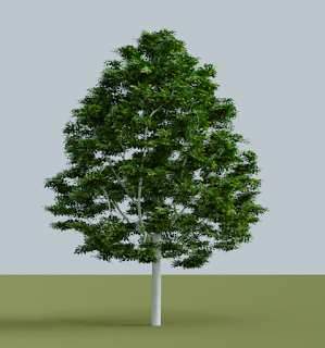
The goal of this article is to document as well as possible what is needed to create realistic trees in de middle distance while using as few rendertime resources as possible.
In a previous article we found that using geometry instead of alpha mapped leaves might be faster to render and in this article we investigate this further and investigate geometry and material choices that allow for realistic trees while minimizing render time and memory consumption.

Realism and middle distance defined

What do we consider to be the 'middle distance'? We are not dealing with image filling close-ups of hero trees but we need more details than a back-plate depicting trees at hundreds of meters away.
For trees I consider the middle distance a distance where we still can see that the tree consists of individual leaves and that when moving we are close enough to see a parallax effect (we see different sides of the tree and perceive it as truly three dimensional.
To achieve realism at this distance then, it is necessary for the tree to be a three dimensional mesh with actual 3D branches in its crown. Also we will still be able to discern the outline of individual leaves (but not very clearly) but surface detail in leaves will not make perceptible difference and neither will small details in the bark texture.
In the sections below I will illustrate the choices I made as I recreate a medium sized red oak (quercus robur) from scratch while keeping this image as a reference.

To create the tree mesh I use my Space Tree Pro add-on but the observations apply to any tree mesh of course.

The reference

The reference photo was shot in fairly light conditions in the afternoon in the spring (May). The tree in question is about 8 meters high and has new spring leaves that are (almost) fully grown. These leaves are individually about 10-12 cm long and all fairly even in color because there is almost no insect, mold or wind damage yet.

We will try to emulate the direction and intensity of the light in the original with a suitable HDRi from HDRI Haven and use filmic color management to approximate these fairly high contrast conditions.
Note that the trunk of this tree is a bit obscured by a metal trellis to guard against damage by goats ;-)
A closeup of the bark shows a fairly uniform grayish texture with comparatively few deeper structures (the tree is about 14 years old).

The camera was at roughly 20-25 meters from the tree.

The crown shape

Most trees have a crown shape that is not a perfect sphere and an oak is no exception. The shape is an egg shape, wider at the bottom than at the top. The crown silhouette is not perfectly smooth still, some bumps and dents are noticeable.
In more mature oak trees these irregularities will result in a more cumulus cloud-like silhouette. Even though the branches themselves are hardly visible due to the leaves, from winter photos we know they have a slightly upward bending habit and are not straight. Note that we do not model every little twig; our leaf particles will be modeled to resemble twigs and not just single leaves.

Foliage density

It is a little bit difficult to find information on the actual number of leaves on a tree of a certain age so we will do this 'by eye'. There are no leaves deep inside the crown but red oaks do not have leaves just at the end of the branches but twigs with leaves are also present deeper into the crown along the branches.

Twigs instead of individual leaves

Leaves are typically connected to small twigs so instead of bunching up all the leaves at points along the branches we create particles with multiple leaves like shown below. Note that at this point we don't bother with the actual shape: the leaves are rectangular and we leave out the actual twig altogether.

Leaf shape

We notice from the initial rendering that at a camera distance of 25m we can see even at this resolution that the leaves are rectangular, so we need to shape these leaves a little bit more.

Geometry vs. alpha mapping

Since we cannot see small details, leaf texture maps are not necessary: instanced geometry is very efficiently rendered, and also real geometry gives us the option to add a real crease and some curvature to the leaves. The final shape we choose is shown in the image below. We create some variations that we place in a group that we can use in a particle system. Remember to use smooth shading on the meshes otherwise you will get sharp reflection boundaries which will give a noisy impression

Leaf material

The leaf material is important but because we cannot see any small details at this distance it will not be necessary to use texture maps, so we will create a simple shader that uses Blender's principled shader node.

Color and roughness

Color and roughness are very important for the look and feel. Because all the leaves on our tree are fresh the color is rather uniform. The leaves are also smooth but not very shiny. The first approximation looks like this:

Variation

Even if we are looking at fairly uniform spring foliage, for visual interest or to get a more summer-like look we might want to add some variation. Because each particle is an object with a unique random number we can use a simple color ramp to drive this color variation. Because each particle has more than one leaf, we give each leaf a unique gray-scale vertex color as well for even more variation.

The node setup we use and the result look like this:


Note that the front and backsides of the leaves are slightly different in real life but we ignore that.

Translucency

If we look at the image now we notice that the coloring is still rather flat, even though the contrast is quite high and we added a bit of color and roughness variation. The main reason for this is that the leaves at the outside receive a lot of light from behind and are a bit translucent. If we add a small fraction of translucency, the whole crown gets a far more dynamic coloring:


Transparency

Translucency implies some transparency as well: the light that is travelling through a leaf and gets through will end up illuminating something else. Transparency will result in longer render times however so we will want to use as few bounces as possible. We use the same noodle as before but add 0.1 transparency in the principled shader:


(Images show 0, 1, 2 and 3 bounces respectively: the difference is hardly noticeable if we add some transparency and more than one bounce is indistinguishable to the human eye)
So we see that transparency is desirable for slightly more light deeper inside the crown but the effect of more than one bounce is limited]

Bark material

With the leaves covered we also need to look at the bark.

Color, roughness and normals

The bark is only really visible on the main trunk. Some color variation is visible at this distance but not much and the bark structure is invisble.

Displacement

The outline of the trunk looks rather smooth and artificial so it will benefit from some extra distortion and even though still experimental in 2.79, micro-displacement is an efficient way to add details to a low poly mesh and break the artificially smooth outline of the trunk. The settings used are the defaults (modifier on the left, material settings on the right):


The shader we use looks like this

Note that we scale everything with the distance to the origin of the mesh [which is at the foot of the trunk), this way small branches will get almost no visible displacement while the foot of the trunk even flares out a little bit, hinting at some hidden root system

Render times

Each effect that we add impacts render times so here is a small summary, all rendered at a resolution of 700x750 pixels at 500 samples with denoising on a GTX970 (the absolute timings will be different on different hardware of course):

Material effects


Featuretime (seconds)
3 transparent bounces174
2 transparent bounces172
1 transparent bounces164
no transparency156
no translucency144

The timings were generated by simply muting the relevant nodes in the material or setting transparent to 0 in the principled shader. Cycles is smart enough to optimize away any unused nodes in the resulting shader.
Since transparency adds quite a bit to the render time, we might skip it all together because as we have seen it is hardly visible in the end result. The 10 extra seconds for translucency however are certainly worth it.

Leaf geometry

We already know that real geometry is faster than using alpha mapped textures, but what about more particles or more detailed geometry? In the images shown until now we each time had 14868 leaves on the tree, each leaf with 448 square faces. If we vary these numbers by changing the number of particles and subdividing the faces in the leaves, we can compare the render times.
number of particles /
number of faces in leaf
100001486820000
448 (1x)154174190
1792 (4x)162183204
7168 (16x)170194226

As we can see, doubling the number of particles does not double the render time. So if we need to create a denser tree crown, adding a few particles does hurt much.
This is even more true for the amount of detail in the leaves: 16 times the number of faces only amounts to approximately 10% extra render time.
The impact on peak memory usage during rendering is minimal: at 7168 faces per particle, 10000 particles peak at 647 MB, and 20000 particles at 651 MB, so with the number of particles we need for a tree the memory usage is hardly a concern.

Conclusion

With our choice of a single transparent bounce but with added translucency we get a nice result. Adding some extra particles or refining the geometry of the leaves does not hurt render times much but there is no need to go overboard as a few extra faces go a long way. No doubt that the realism of the image can be improved even more by proper lighting etc, but I am not an artist so i concentrated on the technical aspects :-)

Freebie

If you like the tree and/or want to experiment with it, you can download the .blend file from my GitHub page. The tree was generated with Space Tree Pro [available on BlenderMarket], so if you own that add-on you can even change its parameters to get different oak trees (the tree parameters are not compatible with my old free space tree add-on)

BlenderMarket spring sale

As there were some technical difficulties BlenderMarket has extended the spring sale until Saturday.

From May 15. til May 18 May 19. BlenderMarket will have its annual spring sale.

Many products will be 25% off their regular price, including my add-ons. So if you had a purchase in mind, this might be fine opportunity to do so!
a full list of everything on sale is available as well.

NodeSet Pro: 2018 Spring Edition

A month ago I introduced the NodeSet Pro add-on on BlenderMarket, an add-on that allows you to quickly create complete node setups from texture sets. In the new Spring 2018 edition I have added significant enhancements, like the options to manipulate collections of textures sets, saving and loading of preference presets and some smaller features like a color ramp node to control the roughness and options to specify your preferred projection mode (when for example you want to work with blended box mapping instead of UV-mapped meshes).

The new features are highlighted in this short video:

The most visible addition is a panel in the tool region that lets you manage collections of textures sets:

If you have additional suggestions to enhance the usability even more, don't hesitate to contact me.

PlaneFit add-on: tiny enhancement

My PlaneFit add-on now features a 2nd menu entry that lets you add the plane as a separate object instead of a part of the mesh.


The addon is available for download from my GitHub repository.
More info on the add-on in this previous article.