Simulating erosion in Blender part IV, addon features.

The addon is getting its shape and the the results are promessing:

(Click to enlarge)

The result on the right was obtained by repeating the (default) settings on the left about 20 times. It is clearly visisble that gullies begin to form, some steep slopes settle at a stable angle and become wider and the central basin starts to fill with silt.

Available options

After selecting the addon and again each time you click the repeat button, the selected mesh is eroded according the selected settings. Each step, all types of erosion (diffusion, avalanches and hydraulic erosion) are iterated a number of times subjected to some probability. By lowering the probabilities in the Probabilities tab certain modes of erosion can be suppressed. The statistics tab shows the actual number of iterations performed after each step.

The ballon help for the options in Thermal erosion and Hydraulic erosion tabs should be self explanatory but careful experimentation gives you a better feel for the possibilities than a lengthy explanation can provide. Don't set the number of iterations too high or each step will take ages; better repeat the the step a few times to gradually get the end result you are looking for. (On my machine, a 6-core, 2.4GHz machine, 10 iterations on a 256x256 mesh typically take 2 ssconds with or without numexpr installed. For larger meshes like 1024x1024 or above, numexpr might help, not only to speed things up but also to reduce memory usage.)

Code availability & feedback

The code is available as an installable .zip file on GitHub. You can install it as a Blender addon by choosing File->User preferences->Addons->Install from file and selecting erosion.zip. Don't forget to enable the addon. The package is dependent on Numpy and having Numexpr and Psutil installed is recomended (the first for serious speedup, the latter for accurate timings, see the opening page of the erosion repository for more info). After the installation the addon is available if you select an object in the 3D View and choose Object->Erode.

Note that if you have installed the erosion addon before, reinstalling it might not get rid of all files in the previous installation. You might try to restart Blender after reinstalling or, if the old version still seems to be there, get rid of the installation directory (typically Your Blender Install Dir\scripts\addons\erosion) and install from scratch.

Besides commenting on this article it might be interesting to check out this BlenderArtists thread.

Previous articles

Articles in this are labeled with the tag erosion. The list up til now consists of:

Simulating erosion in Blender part III, a proper addon

In previous articles (Part I and Part II) I documented my first steps in modeling thermal and hydraulic erosion of meshes in Blender, typically ones created with the ANT landscape generator.

Up til now the code was packaged as a stand alone module meant to be run from the command line. The workflow was cumbersome because exporting a mesh, running the simulation and importing the mesh again is slow, error prone and boring so I went on the convert the code to a proper Blender addon that simply works like any operator in Blender.

This first version only implements the thermal diffusion part but the other functionality (landslides and hydraulic erosion) will follow shortly.

Installation

The code is available on GitHub as a .zip file erosion.zip. Download the file, open Blender and go to File->User preferences->Addons->Install from file and select the .zip file. Don't forget to enable the addon after you've installed it.

The addon depends heavily on the Numpy package and you should have installed this in your Blender python libs for it to work. The Numexpr and Psutil packages are optional but if installed should be in your Blender python directory as well, not just in your system's python dir! How to install external packages is out of scope of this this article (I am strongly in favor of including at least Numpy as part of Blender's bundled python packages but I am afraid it will be difficult to convince the developers :-) but for Windows I have documented what I did on the start page of the GitHub repository.

Usage

After installing the addon and enabling it it is available as an Erode entry in the Object menu of the 3D View as shown in the image below.

The options are in the Toolshelf region as usual and the easiest way to work is to apply the 'repeat last' button from the History tab until you are satisfied with the result. Note that it just works for subdivided planes as created for example by ANT (a closed mesh like a Cube will not work) and the mesh should be in Object mode (currently this is not checked!)

Simulating erosion in Blender part II, fluvial erosion

This second version of my erode.py script adds erosion by water (fluvial erosion, a.k.a. hydraulic erosion). It's not perfect yet, but this first steps already produces some quite interesting results as you can see in the next image:

The image shows a small section of a 256x256 ANT generated landscape. The original is on the left, the eroded version is on the right.(The input file in .raw format and thr commandline parameters to produce the result from the image are provided on GitHub as well, together with the erode script itself.)

Additional options

The script accepts some additional options to control the fluvial erosion (the other options are documented in this previous article).

OptionDefaultDescription
Ka 1.0 Angular dependence
Kc 0.9 Sediment capacity
Kdep 0.0 Deposition rate
Kr 0.1 Rain amount
Ks 0.1 Sediment solubility

Algorithm

Each iteration at each point of the mesh we add an amount of rain to any existing water at that point. Each point also has an amount of suspended sediment and this amount divided by the amount of water gives us the sediment concentration.

By comparing the total heights of rock plus water we calculate how much water flows to and from a point on the mesh and (by multiplying by the sediment concentration) how much sediment is transported.

With these values we adjust the water height and ghe amount if suspended sediment at a given point and recalculate the new sediment concentration. We the compare this concentration to the effective sediment capacity and deposit some sediment if the concentration is higher and dissolve some rock if it is lower.

The effective sediment capacity of flowing water in this model is the product of the base sediment capacity Kc, the sine of the slope a of the heightmap and the speed of the moving water v. How much the slope influences the result is tweaked by the angular dependence Ka:
Kc * sin(Ka * a) * v

Note that faster moving water already has a larger capac2for suspended sediment but on steeper slopes sediment settles less well, effectively increasing the sediment capacith of the water even more.

Reference

Although the code presented here does not use the GPU but relies on Numpy and Numexpr for speed up, the following article proved to be an excellent reference:
Fast Hydraulic Erosion Simulation and Visualization on GPU by Mei et al.
There are however quite some differences, especially in the calculation of the flow field and the order in which the steps if the algorithm are executed.

Future developments

The results so far are promising but we are not there yet. The algorithms need to be fine tuned but I feel experimenting is easier with direct visual feedback so I think I will concentrate on turning this script into a Blender add-on first.

Simulating erosion in Blender part I: Thermal erosion

For some time I wanted to create a script that could erode meshes to complement landscape add-ons like ANT.

The first step is presented here: erode.py, a python script that simulates thermal erosion, i.e. the landslides on steep hill slopes and the gradual breaking up of large boulders by freeze/thaw processes (called diffusion in the code).

It's currently a stand alone script and not yet a proper Blender add-on but it does read and produce raw mesh data that can be exported/imported in Blender (by the raw input/output bundled add-on). It can read hand crafted heightmaps but it is also possible to create some artificial shapes. In its current form the script is intended to verify the algorithms used and get a feel for the simulation parameters.

Code availability and dependencies

The script is available on GitHub. It needs Python 3.2 or newer and depends heavily on NumPy. The code is even multithreaded when the NumExpr package is installed as well and this can make a huge difference for larger grids.

Examples

Some examples are shown below. The first mesh is a mesh generated with ANT. In the second one we applied a few iterations of just the landslide algorithm, which removes the steepest slopes and in the final example we also applied diffusion, softening the landscape as a whole.

Usage

The script isn't very user friendly at the moment but does have a fair number of options:


usage: erode.py [-h] [-I ITERATIONS] [-Kd KD] [-Kh KH] [-Kp KP] [-ri] [-ro]
[-i] [-t] [-infile INFILE] [-outfile OUTFILE] [-Gn GRIDSIZE]
[-Gp GRIDPEAK] [-Gs GRIDSHELF] [-Gm GRIDMESA] [-Gr GRIDRANDOM]
[-m THREADS] [-u] [-a] [-n]

Erode a terrain while assuming zero boundary conditions.

optional arguments:
-h, --help show this help message and exit

-I ITERATIONS the number of iterations
-Kd KD Diffusion constant
-Kh KH Maximum stable cliff height
-Kp KP Avalanche probability for unstable cliffs

-ri use Blender raw format for input
-ro use Blender raw format for output
-i use an inputfile (instead of just a synthesized grid)
-infile INFILE input filename
-outfile OUTFILE output filename
-t do not write anything to an output file

-Gn GRIDSIZE Gridsize (always square)
-Gp GRIDPEAK Add peak with given height
-Gs GRIDSHELF Add shelf with given height
-Gm GRIDMESA Add mesa with given height
-Gr GRIDRANDOM Add random values between 0 and given value

-m THREADS number of threads to use
-u perfom unittests
-a show some statistics of input and output meshes
-n use numexpr optimizations

Exporting and using an ANT generated mesh

Create a landscape mesh
For example with ANT but of course you can sculpt one as well or import a DEM
Export the mesh
File->Export->Raw. Make sure you enabled the add-on
Erode it
See example commandline below
Import the mesh
File->Import->Raw

Assuming you exported the grid to a file called untitled.raw, you could erode that file and put the result in a file called out.raw using the following command line:


python erode.py -Kd 0.001 -Kh 0.03 -i -infile untitled.raw -ri -outfile out.raw -ro -I 10

(Which model parameters (especially Kh) to use depends of course on the input mesh.)

Future developments/Roadmap

Erosion due to whethering isn't all that interesting in itself but serves to test the basic data structures in the script. Water erosion is the final goal so the roadmap for this script is short: fluvial erosion (creation of canyons and gullies and the deposition of sediment due to rain) will be next and when that works I'll rework the script to a proper addon. After that we'll see if there is demand for other features. I would like to add meandering but based on my current research I think that's quite some effort so I'll see if I can find the time.

Reference

This work was inspired by the work of Musgrave et al.. A more in depth an physically meaningful source worth reading is textbook by Pelletier.

Drawing cubic splines in OSL

Some time ago I wrote about a routine to calculate the closest distance to a quadratic bezier spline and recently I reused this routine again in a slightly optimized form to create wiggles.
Being able to calculate the closest distance to a quadratic spline is useful but I really wanted to use cubic splines because they offer more control, allowing for easier ways to create nice shapes.

update: made the code 10% faster by making it 2D only. The GitHub version relects that change but original code can be used by removing a single macro
Warning; long read ahead :-) The first section describes how to use the shader and where to download the code and is pretty short. The second section dives deep into the code and is definitely not an easy read, sorry for that but fortunately there is no need to go that deep if you know what a cubic spline is and just want to use the code.
If you would like to know more about programming OSL you might be interested in my book "Open Shading Language for Blender". More on the availability of this book and a sample can be found on this page.

The shader

The approach to finding the distance to a cubic spline is the same in principle as for a quadratic spline: find all values for t that satify the relation dB(t)/dt . (B(t) - P) = 0, or in English: those values of t whre the tangent to the spline is perpendicular to the vector pointing to the point being shaded (remember that the dot product of two vectors is zero if they are perpendicular).
For a quadratic bezier curve the equation to solve is cubic and is quite simple but for a cubic bezier curve this is a fifth order equation for which there is no analytical solution. And although cubic splines are used everwhere (for example in fonts) a numerical solution for this problem was surprisingly hard to find.
Fortunately after some serious searching the Graphic Gems series of books proved again to be incredible useful, specifically "A Bezier Curve-Based Root-Finder" by Philip J. Schneider.
The original code is in C so it neede quite some work to convert it to OSL. Normally converting C code to OSL is pretty straightforward but this code uses multidimensional arrays and recursion, both unknown to OSL. On the plus side, OSL's native point type and built-in dot() make for a lot less code.

Code availability and node setup

My implementation (with a sample shader in the same file) is available on GitHub. The node setup used to create the heart shape is shown below, it is made of two mirrored splines:

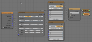
The values for the control points are:P0 = ( 0.5, 0.1, 0.0)
P1 = (-0.5, 0.7, 0.0)
P2 = ( 0.4, 1.2, 0.0)
P3 = ( 0.5, 0.8, 0.0)

Code explanation

I am not going to list all of the code because it's way to long and rather boring but I will tell some more about the FindRoots() which is nontrivial and needed to be reimplemented in a non-recursive form.
The general idea of the shader to cast the fifth order equation whose roots we'd like to find in a form that is itself a bezier curve (I.e. a bernstein polynomial) and exploit the specific properties of a bezier curve to efficiently find the roots.
The mathematical specifics are explained very well in Schneider's article so let us just look at the code:
#define POP wtop+=6;wn--

int FindRoots(point w0[6], float t[5]){
  point w[STACKSIZE];
  int wtop=0;
  int wend=0;
  int wn=0;
  for(int k=0;k<6 br="" k="" w0="" w="" wend="">  wn++;
  int nc=0;
  while(wn>0){
    //printf("[%d]",wn);
    int cc=CrossingCount(w,wtop); // w[:5]
    if(cc==0){
      POP;
      continue;
    }
    if(cc==1){
      if(wn>=MAXDEPTH){
        t[nc++]= (w[wtop][0]+w[wtop+5][0])/2;
        //printf(" MAX ");
        POP;
        continue;
      }
      if(ControlPolygonFlatEnough(w,wtop)){ // w[:5]
        t[nc++]= ComputeXIntercept(w,wtop);
        //printf(" FLAT (%.1f | %.1f)",w[wtop],w[wtop+5]);
        POP;
        continue;
      }
    }
    // not flat or more than one crossing
    DeCasteljau(w,0.5,wtop,wend);  //left=[wend:wend+5], right=[wend+6;wend+11]
    for(int k=0;k<6 br="" k="" w="" wend="" wtop="">    wn++; wend+=6;
  }
  return nc;
}
A fifth order bezier curve has 6 control points and at most 5 roots. The control points are passed as the w0 argument and the t array will receive the root values. The function's return value will be the number of roots found.
The central idea of this algorithm is to find a segment of the curve that crosses the x-axis just once and then determine the intercept, i.e. a root. To achieve this the spline is subdived into to halves, each again a fifth order spline, until such segment contains a single crossing.
Because OSL doesn't support recursion, we have to maintain a stack of control points ourselves and that's where the w array comes in.
Starting with the for-loop in line 8 we transfer the initial set of 6 control points to the stack and adjust wn to reflect that we now have one set on the stack. At this point wtop (the index of the first control point in the topmost set) is 0, and wend (the index of the first free slot in w) is 6. nc holds the number of roots found sofar.
Next we iterate as long as there is a set of control points on the stack (line 11). We caculate how many times the curve defined by this set crosses the x-axis. If there is no crossing there is no root in this curve so we pop the set of the stack and continue.
If there is a single root and we have recursed deep enough we simply approximate the root as lying halfway between the x-coordinates of the first and last control points and pop the set (line 20). If there is room to recurse we check whether the set of control points is "flat enough" (line 25) and if so compute the intercept with the x-axis of the line between the first and last control point. We store this root and pop the set of control points (see Schneider's article or the original source code to see what is meant by "flat enough").
If the control points are not "flat enough" or we have more than one root in this curve, we split the curve in two using DeCasteljau's method (line 33). The function will produce two sets of six control points at position wend in the w array. The save space we copy the second set to top of the stack (because the control points for the original curve are no longer needed), which means we only have to increase the stacksize wn by one.
Finally, if we run out of the while-loop we simply return the number of roots found.

Speed

Now you might think that all this recursion and the numerous calculations would be very slow but you will be surprised. The function seldom needs to recurse very deep because the accuracy used to determine if a curve is "flat enough" need not be that good (we can't see differences much less than a pixel). On my machine this means that I can tweak the node setup for the example image at interactive speeds if I set the number of preview samples to 1.
There is however plenty of room for optimization, especially in areas were we do calculations with 3D points. If we only want to work in 2D we might save up to 30% on unnecessary calculations.

Creating unique snowflakes with OSL

Falling snowflakes are easy enough to dimulate in Blender with a particle system but if quite a few of them might be seen fairly close up, the real challenge is in making sure each one is unique.

The shader presented in this article will create a unique snowflake for each value of its Seed. Using the object info node we may obtain a unique random number for each object that we may use for this purpose as we will see when we examine the node setup.

Snowflakes

The code below defines the following utility functions;
hex
this function will produce the x and y coordinates of a point as it is rotated through the six segments of a hexagon
in_hexagon
this function will return a non zero value if a point lies within a hexagon
pattern
this function does the real work. It returns non zero if a point is positioned within a number of hexagons that are randomly positioned along the x-axis. It also draws a connecting rod that extends as far as the farthest hexagon.
The body of the shader itself just copies the position being shaded along a hexagon and then calls pattern(). Note that because we expect uv-coordinates for a simple square (I.e in de range [0,1], we transform these coordinates so that the center is at (0.5, 0.5) [line 68].
#define SLOPE 1/sqrt(3)
#define SIDE sqrt(.75)
#define D60c cos(radians(60))
#define D60s sin(radians(60))
 
void hex(float x, float y, output float hx[6], output float hy[6]){
  hx[0]=x;
  hy[0]=y;
  hx[1]=x*D60c-y*D60s;
  hy[1]=y*D60c+x*D60s;
  hx[2]=x*D60c+y*D60s;;
  hy[2]=y*D60c-x*D60s;
  hx[3]=-hx[0];
  hy[3]=-hy[0];
  hx[4]=-hx[1];
  hy[4]=-hy[1];
  hx[5]=-hx[2];
  hy[5]=-hy[2];
}

int in_hexagon(
  float px, float py, 
  float cx, float cy, float r, 
  output float d
){
  d=hypot(px-cx,py-cy);
  if(d>r){ return 0; }
  float hx[6],hy[6];
  hex(px-cx, py-cy, hx, hy);
  for(int h=0; h < 6; h++){
    if((abs(hy[h]) < SLOPE*hx[h]) && (hx[h]< r*SIDE)){
      d=abs(hx[h]);
      return 1;
    }
  }
  return 0;
}

#define CELL noise("cell",seed++)

float pattern(float x, float y, int Seed, int Kernels){
  int seed=Seed;
  int n=(int)(1+Kernels*CELL);
  float hx=0, maxx=0;
  for(int f=0; f < n; f++){
    float hy=0;
    float r=0.2*CELL;
    float d;
    if(in_hexagon(x,y, hx,hy,r, d)){
      return d;
    }
    hx=SIDE*CELL;
    if(hx>maxx){maxx=hx;}
  }
  if(x < maxx && abs(y) < 0.01){ return 1; }
}

shader snowflake(
  point Pos=P,

  int Seed=0,
  int Kernels=15,
  
  output float Fac=0
){
  float hx[6],hy[6];

  hex(2*(Pos[0]-0.5), 2*(Pos[1]-0.5), hx, hy);

  for(int h=0; h<6 br="" fac="=0;" h="">    if(abs(hy[h]) < SLOPE*hx[h]){
      Fac=pattern(hx[h],hy[h],Seed, Kernels);
    }
  }
}

Example node setup

The node setup used to shade the particles in the image at the start of this article looks like this:

The random value from the object info node lies in the range [0,1], so we multiply it by a large value to get a unique integer.The output of the shader node is checked to see if it is non-zero. if so we use a group of shaders to mimic ice, otherwise a transparent shader. The Fac output may vary smoothly so we use a color ramp node with constant interpolation the create stepped values that we can use to drive an ice-like bump pattern. The Kernels input determines how many random hexagons are within each snow flake, so this essentially controles how dense the flakes look.

Code availability

You can copy the code from the listing above but you may also dowload it from GitHub.
If you would like to know more about programming OSL you might be interested in my book "Open Shading Language for Blender". More on the availability of this book and a sample can be found on this page.

Full book review: Blender 3D printing essentials

Last weekend I had the pleasure to read Blender 3D printing esentials by Gordon Fisher.

Gordon previously authored Blender 3D Basics and his experience and subject skill is clearly shown in this new short book 3D printing. The book is Blender specific of course but pretty much 3d-printer agnostic, so it's useful not only for printer owners but also for people who want to use online print shops.

Pros:

short
about 100 pages real content. Clear language as well, so you won't need much time to get up to speed

to the point
it won't tell you much about modelling as such but does show what elements of modelling need extra care when preparing a model for printing and how to fix problems

complete
all you need to know for most common printing materials and printing techniques but of course with new materials becoming available every day you'll have to check the material specifications for things like minimum wall thickness if you want to try a new material but that is not a critique on the book. On the contrary, it does an excellent job of describing things like what influences surface detail, why wall thickness is important and when and how to deal with overhang.

good description of essential tools
Blender's 3D printing toolkit and mesh analysis tools are covered well and the use of the protractor tool (to measure distance and angles in your model) is explained very clearly.

Cons:

uv-unwrapping and texture painting
(for printers that support multicolored models) would have benefited from more in depth attention as these subjects are generally considered difficult by beginners

the price
I personally feel that the €13,56 list price for a 100 page e-book is steep, not to mention the almost €26,- price tag for the print version, but of course online retailers may give you a better deal.

Conclusion

Good book, well written. Based on the content alone I would give it 4.5 out of 5 stars but the unrealistic price tags lowers that to 4.

If you would like to know more about programming OSL you might be interested in my book "Open Shading Language for Blender". More on the availability of this book and a sample can be found on this page.