Generate floor boards quick and simple

I am updating this addon, check for an update this article.

I am currently enrolled in Andrew Price's Architecture Academy and in one of his tutorials he mentioned how easy it would be to have a simple script that could create floor boards suitable for architectural renders like those available in some other modelling packages. He even thought about asking someone to develop it but for some reason or other it never came te be.

Add Floor Boards

Because I think it would make a useful addition to the ArchViz' modeller 's tool set I put together a simple script Add Floor Boards. Once installed it can be found in the Add->Mesh menu at the to of the 3D view. Slap on a decent wood shader and you have a floor with real geometry in a few seconds.

The object that is generated by the script is a simple collection of rectangular faces adorned with a solidify and a bevel modifier so you can tweak some stuff even after the tool properties are no longer accessible.

Installation

  • Download the script from GitHub
  • Click File->User Preferences->Addons and click the install script from file
  • Don't forget to enable the add-on, it can be found in the Add Mesh section

Usage

After clicking Add->Mesh->Add Floor Board a default floor board is generated. The tool options should be self explanatory and are shown below:

Note that the measures are in blender units and the defaults reflect typical oak boards available at my local floor board dealer and are denoted in meters. (If you do archviz work it makes sense tp select some units in the scene options). Note that the variations in length and width are added to the base measurements so set them to zero if you want comlletely regular planks (a fixed width is quite common, a fixed length not so much as it leads to waste).

Blender addon to setup image based lighting (IBL) nodes in Cycles

setting up image based lighting (IBL) in Cycles isn't all that difficult but creating a versatile setup requires a lot of repetitive actions that lends itself well to automation. In this article I present a simple add-on that may be accessed from the Add menu in the node editor to quickly set up all the nodes for environment lighting.
Note: as of 2015/03/13 a bug fix release is available on GitHub.

The SIBL archive

One of the resources I find myself using quite often is the SIBL archive. Each archive is basically a directory (commonly packed as a .zip file) that contains both a high resolution backplate and HDR environment and reflection maps. It also contains an .ibl file that documents the resources available in the .zip file. The add-on uses this .ibl file to create all necessary nodes and references to the images. I am not sure how widely accepted the SIBL format is, but the add-on can also be used by simply selecting a .jpg and a .hdr file instead of a .ibl file so you are not restricted to just SIBL files.

Installation


Download the add-on
It is available on Github as a single file sibl.py. You can directly save it to your download directory via this link.
Install in Blender
Open the add-ons section of Blenders User Preferences and click Add external add-on. Select the downloaded file and click install. After installation you may find it in the Node section where you can activate it.

Usage

With a SIBL archive

Enable the add-on
In the add-ons section of the user preferences. It sits in the Node category.
Download a SIBL archive
Unzip the archive
Go to the World nodes
Click the world icon in the node editor.
Click Add -> Sibl Environment Setup
Select the .ibl file
Click Add Environment

With separate files

Enable the add-on
In the add-ons section of the user preferences. It sits in the Node category.
Go to the World nodes
Click the world icon in the node //editor.
Click Add -> General Environment Setup
Select one or two files
If you select more than one file, a file with a .hdr extension will be used as the environment lighting and the other one as the backplate.
Click Add Environment
After selecting the files the node setup will be displayed in the node editor. If there were any issues with the .hdr or backplate images the corresponding environment texture node is colored red. This may happen if the file is unreadable for some reason or if the the .ibl file points to non existing files.

Options

When the file selector is opened to allow you to select a file, some options are available in a panel on the left of the list of files:
Use reflection map
This one is only present when opening a .ibl file. It selects a higher resolution environment map suitable for glossy reflections (if available). You probably should only use this if you want to see the environment reflected in glossy surfaces because a reflection .hdr uses a lot more memory than a low resolution .hdr environment map.
Clear node tree
Uncheck this if you want to keep any existing nodes in the world node tree. If unchecked a world output node will be reused if present, as are any texture coordinate and light path nodes. Other nodes are untouched.

Implementation details

While developing this add-on I noticed that the [Environment] section in some .ibl files was spelled without an n. This is probably a bug but this add-on accepts both spellings. (An .ibl file is formatted as an .ini file, a common file format on windows and easily parsable with Python's configparser module.
All meta-data in .ibl files is ignored. This means any sun or additional key lights defined in the file are ignored. Also, all image files are currently assumed to be spherical (a.k.a. equirectangular or LatLong format, Blender's default mapping for environment textures). This means that light probe maps are currently not supported.

An OSL wood shader with knots for Blender Cycles

In a previous article I presented a shader that could be used to create the impression of knots in wood. This was accomplished by warping the texture coordinates around randomly distributed points in space.

Knots however do not resemble spheres but are more like cylinders that are cut under a slight angle. This distinction is not that important but for completeness sake we present this new implementation here together with a node setup that combines these knots with the wood shader we presented a while ago. An example result is shown below.

Code and example node setup

The implementation differs from the previous one in generating random lines (represented by a random point plus a random direction) instead of points. The texture coordinates are bent proportional to the distance to the closest point on this random line, so the bend() is a little bit more complicated than before.


vector random_sphere(point p, int n, float zdistribution){
float t = M_2PI*noise("cell",p,n*2+0);
float u = 2*noise("cell",p,n*2+1)-1;
float s,c,a;
sincos(t,s,c);
a = sqrt(1-u*u);
float x = a*c;
float y = a*s;
float z = u*zdistribution;
return vector(x,y,z);
}

int bend(vector p, vector k, vector kv, float r, float a, float m, output vector B){
vector pk = k - p;
vector t = dot(pk,kv)/dot(kv,kv);
vector D = k + t * kv - p;
float L = length(D);
if( L < r ){
float c = L/r;
float d = m * pow( 1 - c , a);
if( d < L ){
B = d * normalize(D);
return 1;
}else{
B = D;
return 2;
}
}
return 0;
}

shader knot(
vector Pos = P,
float Scale = 1.5,

float R = 2.9,
float Falloff = 2,
float Strength = 1,
float Knots=0.1,
float Z=1,

output vector Vec = P,
output float Fac = 0
){
vector p = Scale * Pos;
vector sdp = 0;

float TR = ceil(R);
for(float dx=-TR; dx <= TR; dx++){
for(float dy=-TR; dy <= TR; dy++){
for(float dz=-TR; dz <= TR; dz++){
vector ip = floor(p)+vector(dx,dy,dz);
for(int ik=0; ik < (int)Knots; ik++){
vector k = noise("cell",ip,ik);
vector kv= random_sphere(ip,ik+1000,Z);
vector dp= 0;
int ret = bend(p,ip+k,kv,R,Falloff,Strength,dp);
if(ret != 0){
Fac=max(Fac,ret==2);
sdp+=dp;
}
}
if( noise("cell",ip,-1) < mod(Knots,1.0) ){
vector k = noise("cell",ip,-2);
vector kv= random_sphere(ip,998,Z);
vector dp= 0;
int ret = bend(p,ip+k,kv,R,Falloff,Strength,dp);
if(ret != 0){
Fac=max(Fac,ret==2);
sdp+=dp;
}
}
}
}
}
if( Fac < 1 ){
Vec = p + sdp;
}else{
Vec = sdp;
}
}
Note that the function random_sphere() is modified from the one presented in a previous article to bias the vectors that are returned. This allows us to tweak the orientation of the generated knots, which might give more realisted results because branches (the source of the knots) are not pointing in all directions from the stem.

The node setup used to create the material in the example image is shown below (click to enlarge).

Room for improvement

The distribution of the knots might be convincing enough for our purposes but the material is now just another (darker) wood mzterial, rings and all. Quits a number of wood knots do look like that but a significant fraction shows characteristic radial cracks. This is caused when the wood is dried because the material properties of the knot are different from the surrounding wood. It would be nice if we could implement this in some way as well.

Random points on a unit sphere in OSL, code and benchmarks

In preparation to adapting the wood knot shader to have randomly oriented cylindrical knots rather than spherical knots I needed a function that generates vectors that are uniformly distributed over the surface of a unit sphere. This is not as simple as creating a vector with three random components but several methods exist that will produce vectors with a correct distribution.

A straight forward method (implemented in the function random_sphere() shown below) consists of generating correctly distributed spherical coordinates and the converting them to cartesian coordinates. This works fine but because trigonometric functions (like acos() and sincos()) used here) may be expensive, several alternatives exist that do not use these functions.

In the code presented here we have implemented the methods of Marsaglia (random_sphere1()) and Cook (random_sphere2()). Both are rejection methods: they discard some random numbers when they would lead to invalid vectors. This is wasteful so the question is: are these methods really more efficient on modern hardware where trigonometric functions are implemented as cpu operations?

Some timings

The timings presented below were measured on a 64-bit Amd 6-core cpu with the shader provided below. They might be completely different for other CPUs and probably even more so once OSL shaders will be able to run on a GPU.

nrandom_sphererandom_sphere1 random_sphere2
100 3.6 3.4 7.5
500 10.4 10.1 -
First thing to note is that the timings for 100 and 500 vectors do not scale proportionally because some of the dots we draw with our shader overlap, effectively reducing the number of vectors we have to generate for each shading sample. The other thing is that random_sphere2 is much slower than the other implementations, probably because we generate more random numbers and reject a lot more combinations.

As for the difference between the other two methods: the difference is probably significant but too small to make a real difference on my CPU. I'll probably check again when I get another CPU or OSL shaders will run on a GPU, but for now I stick with the most straightforward method.

Code and node setup


// generate random unit vectors randomly distributed over a sphere
// straight forward method
vector random_sphere(point p, int n){
float t = M_2PI*noise("cell",p,n*2+0);
float u = 2*noise("cell",p,n*2+1)-1;
float s,c,a;
sincos(t,s,c);
a = sqrt(1-u*u);
float x = a*c;
float y = a*s;
float z = u;
return vector(x,y,z);
}

// marsaglia's method
vector random_sphere1(point p, int m){
vector v = 0;
float repeat = 0;
int n = m + 1;
while(1){
repeat++;
float r0 = 2*noise("cell",p,repeat*n*2+0)-1;
float r1 = 2*noise("cell",p,repeat*n*2+1)-1;
float r02 = r0*r0;
float r12 = r1*r1;
float sr2 = r02 + r12;
if( sr2 < 1 ){
float x = 2*r0*sqrt(1-r02-r12);
float y = 2*r1*sqrt(1-r02-r12);
float z = 1-2*sr2;
v = vector(x,y,z);
break;
}
}
return v;
}

// cook's method
vector random_sphere2(point p, int m){
vector v = 0;
float repeat = 0;
int n = m + 1;
while(1){
repeat++;
float r0 = 2*noise("cell",p,repeat*n*4+0)-1;
float r1 = 2*noise("cell",p,repeat*n*4+1)-1;
float r2 = 2*noise("cell",p,repeat*n*4+2)-1;
float r3 = 2*noise("cell",p,repeat*n*4+3)-1;
float r02 = r0*r0;
float r12 = r1*r1;
float r22 = r2*r2;
float r32 = r3*r3;
float sr2 = r02 + r12 + r22 + r32;
if( sr2 < 1 ){
float x = 2*(r1*r3 + r0*r2)/sr2;
float y = 2*(r2*r3 - r0*r1)/sr2;
float z = (r02 + r32 - r12 - r22)/sr2;
v = vector(x,y,z);
break;
}
}
return v;
}

shader sphere_test(
vector p = P,
int n = 100,
float R = 0.03,
int method = 0,

output float Fac = 0
){
for(int i=0; i < n; i++){
vector v = 0;
if( method == 0 ){
v= random_sphere(point(0,0,0),i);
}else if( method == 1){
v= random_sphere1(point(0,0,0),i);
}else{
v= random_sphere2(point(0,0,0),i);
}
if( distance(point(0,0,0),1000*v,p ) < R ){
Fac = 1;
break;
}
}
}

The way we generate random numbers might seem strange but not only do we want to be able to generate any number of vectors for a given cell but in the rejection methods we also want to be able to generate replacements that are guaranteed to be different, hence the multiplication by the number of times we have to repeat.

The image shows the node setup used to verify the shader and time the different implementtations

An OSL wood knot shader

Back in january I presented a wood shader that produces decent results but one of things that was missing was a way to add realistic knots to planks. In this article a present a shader that is meant as a first step in producing knots. It is not a finished shader yet, but it is fully functional as a texture warping tool and in a future article I might detail how to combine it with a wood shader and a shader to texture the inside of the knot properly. Because that will take some time so I thought it better to present it as a WIP as I am currently unable to spend more than a few minutes behind my desk (and there's no Blender for Android alas).

Warping space

The idea is quite simple and might be adaptable to more than just producing knots: we distribute points randomly and warp the position coordinates around these points. These warped coordinates are then used as the basis for a texture. In the example image we use the warped coordinates as the input to a bands texture:

As you can see the bands of the texture seem to flow around the knots as if they were repelled by them and in fact that is pretty much how the algorithm works.

Implementation


int bend(vector p, vector k, float r, float a, float m, output vector B){
vector D = k - p;
float L = length(D);
if( L < r ){
float c = L/r;
float d = m * pow( 1 - c , a);
if( d < L ){
B = d * normalize(D);
return 1;
}else{
B = D;
return 2;
}
}
return 0;
}

shader knot(
vector Pos = P,
float Scale = 5,

float R = 0.8,
float Falloff = 1,
float Strength = 0.9,
float Knots=0.5,

output vector Vec = P,
output float Fac = 0
){
vector p = Scale * Pos;
vector sdp = 0;

float TR = ceil(R);
for(float dx=-TR; dx <= TR; dx++){
for(float dy=-TR; dy <= TR; dy++){
for(float dz=-TR; dz <= TR; dz++){
vector ip = floor(p)+vector(dx,dy,dz);
for(int ik=0; ik < (int)Knots; ik++){
vector k = noise("cell",ip,ik);
vector dp= 0;
int ret = bend(p,ip+k,R,Falloff,Strength,dp);
if(ret != 0){
Fac=max(Fac,ret==2);
sdp+=dp;
}
}
if( noise("cell",ip,-1) < mod(Knots,1.0) ){
vector k = noise("cell",ip,-2);
vector dp= 0;
int ret = bend(p,ip+k,R,Falloff,Strength,dp);
if(ret != 0){
Fac=max(Fac,ret==2);
sdp+=dp;
}
}
}
}
}
if( Fac < 1 ){
Vec = p + sdp;
}else{
Vec = sdp;
}
}
The magic is in the bend() function. It calculates the difference vector from the point being shaded to the center of the repulsion. If the distance is short enough, a translation vector is returned that is a distance dependent fraction of the difference vector. It takes some thinking to see that in order to create the illusion of repulsion we actually have to replace the point being shaded towards the center of repulsion: remember that at the point we are shading we want to see the lines closer to the center.

When we calculate the translation towards the center and we are close enough to it, we might overshoot the center point. In which case we return a value of 2, signalling we are inside the knot and return not the translated shading point but the vector pointing to the center (which might be useful to render some concentric pattern in the knot).

The shader itself is nothing more than checking if we might be in range of one of the randomly distributed points and calling the bend() function to do the actual work. We do allow for a fractional number of knots per unit cell, in which case the fraction acts as the probability that a knot might occur.

Room for improvement

Obviously knots are not spherical marbles embedded randomly in some wood but as the remnants of branches they are more reminiscent of stubby cylinders which might be better modeled by determining the distance to a randomly oriented line segment instead, something I intend to implement in the near future.

Another area that needs attention is to way the inside of the knot appears. In the example setup we produced some concentric circles but a real knot is a bit more complex than that.

OSL debugging tips

The other day I was debugging a shader that didn't produce the results I expected, in fact it didn't produce any output at all. In its basic form it resembled the following shader:


shader S(
vector position = P,

output color Color = 0
){
... many calculations ...
if( ... some condition ...){ Color = 1; }
}

When I hooked this shader up in some node setup, I'd expected it to produce a pattern but all I got was a uniform black. Obviously the condition was never true and Color was never assigned a value of 1. So I had to determine what the values of some intermediate values were to get an idea why the if statement didn't fire.

So I inserted a printf() call:


shader S(
vector position = P,

output color Color = 0
){
... many calculations ...
printf("%.2f\n",position);
if( ... some condition ...){ Color = 1; }
}

I clicked the recompile button, looked in the console and ... nothing was printed! To be 100% sure that the shader was evaluated I changed it to:


shader S(
vector position = P,

output color Color = 0
){
... many calculations ...
printf("%.2f\n",position);
if( ... some condition ...){ Color = 1; }
Color = 0.5;
}

Now the node setup produced the expected shade of gray, so it was hooked up correctly and was indeed being executed but more surprisingly, the console showed the printf output.

This baffled me: if I commented out the final assignment to Color, the printf() wasn't executed. I thought I found a bug in OSL and reported it. But was it?

Constant folding

It turned out that this is intended behavior. The OSL compiler is a clever piece of software and does its best to reduce unnecessary calculations. One of the tricks it employs is called constant folding, a method in common use in many compilers. Basically it tries to calculate at compile time anything that can be compiled, for example:

twopi = 2 * 3.14;fourpi = 2 * twopi;

becomes after compilation:

twopi = 6.28;fourpi = 12.56;

This keeps your code readable but reduces actual calculation at runtime. And this can lead to significant speedups when you are shading milions of samples.

OSL has a lot more of these tricks up its sleeve and can reduce quite complex expressions, even removing branches from if/else statements. But it goes a step further still. If the compiler detects that none of the output values is changed from its default by a shader, this shader is not executed at all.

For my example shader this implies that because the condition in the if statement is apparently based on things that can be calculated at compile time and never true, the if statement is optimized away. The result of this is that no output value will ever be changed by this shader and so the whole shader is optimized away, even if we put printf(), warning() or error() calls in this shader, because statements that produce side effects only and do not contribute to the output of the shader are not by themselves considered enough to keep an if/else branch or even a shader from being optimized away.

Debugging OSL code

Now if we want to debug some code we might have a problem because simply inserting a printf() call is no guarantee that the information we are interested in will be printed. Also, assigning a value to an output socket might not be enough:


shader S(
vector position=P,

output color Color=0
){
...
printf(.....);
Color = 1;
Color = position[0];
}

Neither of the last two statements will ensure that the printf() call is executed. The first one us an assigment of a constant and can be calculated at compile time. The last one only depends on the input and can be 'hardwired', that is, there is no need to execute the shader; the compiler can simply connect input and output.

So if we want to make sure the printf() executes, we need an assignment to Color that cannot be calculated at compile time, for example one of:

Color = position[0]>0;
Color = rand();

Another option is to create an extra output socket just for debugging and assign the variable that you are interested in to this socket. If you connect it to a diffuse shader there is a lot you can tell based on the color, but of course not all variables are suitable for this approach (strings to name one).

New debugging options

From release r57660 (download it from the daily builds, I tested the 64bit windows version) you can disable OSL optimizations by assigning a value to the OSL_OPTIONS environment variable. If you use Windows this can be done like this:

  • open a command prompt
  • set the variable (don't use quotes)
    set OSL_OPTIONS=optimize=0
  • run Blender from the command line
    C:\path\to\blender.exe
  • don't forget to recompile your OSL shader
On unix-like systems you start from an xterm or equivalent and type export OSL_OPTIONS="optimize=0"
path/to/blender
(if you do not use bash but tcsh use setenv instead of export). Setting these variables is local to the command prompt/xterm you are working in so when you exit Blender and close the command prompt the optimization override will be gone. Changing the enviroment on a more global level is not recommended. Also when you're done it might be a good idea to remove all printf calls from you production code because printing to a console is extremely slow. You might still want to print information in exceptional situations but you might consider using error() for that purpose.

Conclusion

In many cases using printf() calls to debug your OSL shaders is still the method of choice but if nothing shows up on the console make sure that these calls are not optimized away.

Working with the incidence vector in OSL

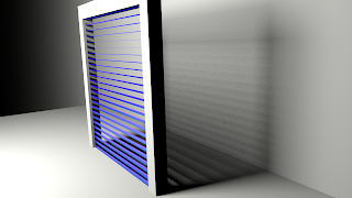
The fact that in OSL we have the incidence vector I available has proven its utility already in the many cool toon and carpaint shaders people have implemented. In this article we take this concept a bit further and create a shader that does not change it lighting model as a function of the angle between incidence vector and normal but changes its complete behavior depending on the angle between incidence vector an object orientation, allowing us the model a 3D-object (Venetian blinds) with just a 2D-tecture.

Lenticular printing

The idea of providing a different image based on the viewing angle is not new and is fact readily available in traditional media under the name Lenticular printing.But in OSL we are able to act on any incidence vector, not just the one from the camera. This means for example that shadow rays act as they should and that we can make our material transparent in places to let it cast correct shadows.
In the sample image and in the video we used this trick to render venetian blinds as seen from different position with just s single plane.
The concept is simple: the horizontal slats of the blinds appear taller when seen from an angle so we calculate the angle between the incidence vector and the x-axis (because unfortunately there is no attribute object:rotation to determine the up axis of an object) and divide that by maximum angle that would let us see something through the blinds. That fraction is used to paint part of a horizontal strip representing a slat. Finally we replace the shading normal by one that is perpendicular to the slat allowing for s bit of a curve across the slat:
surface venetianblinds(
  point Pos = P,
  float Spacing = 0.1,
  float Width = 0.1,
  float Curve = 0.2,
  
  output float Fac = 0,
  output float Top = 0,
  output normal Normal = N
){
  Top = dot(I,vector(0,0,1))>0;
  
  float maxangle = atan(Spacing/Width);
  float angle = abs(M_PI_2-acos(dot(normalize(-I),vector(0,0,1))));

  float height = Spacing;
  // TODO we should look at the sign here to prevent 'flip'
  if (angle < maxangle){ height *= angle/maxangle; }

  float z = mod(Pos[2],Spacing);
  Fac = (z < height);
  
  if(z< height){
    Normal = normalize(vector(0,0,1)+N*Curve*(height/2-z)/height);
  }
  
}

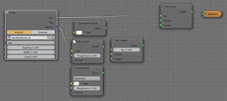
Example node setup

The node setup used to render both the still and the video looks like this: This material is applied to a simple plane. The lighting consists of a single mesh light on the left.