one of the issues that bothered me about my new tree add-on was that applying the skin modifier to flesh out the branch skeleton was incredibly slow, especially for larger trees. I therefore decided i'd try writing my own skinning routine and the results are quite promising: a factor 10 or more for moderately sized trees.
The new version (0.0.7) is as usual available on GitHub. How to use and install this add-on is documented in previous articles: IIIIIIIV. The new skinning method is the default if you uncheck the no modifiers checkbox but if you like you can still select Blenders skin modifier from the drop down as shown on the right. (This can also be done later because we leave the skeleton itself intact; as it only consists of edges it won't show up in renders but you could use it to add any modifier later on).
Timings
The table below lists some timings for my computer, all values were left to their defaults except for the number of endpoints:
Timings in seconds for generating a tree skeleton
Endpoints
No modifier
Own skinning
Blenders skinmod
100
0.02
0.04
0.46
200
0.04
0.07
0.74
400
0.08
0.16
1.51
400
0.56
0.87
14.43
The last line shows the results for a fair sized, bushy tree (400 endpoints, but with the internode length and kill distances reduced to 0.5 and 2.5 respectively and with 3000 extra endpoints per 1000 iterations). The difference between less than a second and more than 14 seconds is the difference between comfortable modelling and frustration, and there is still some room for improvement because the code is still riddled with print statements. There are three factors that help to speed up the skinning operation compared to blenders built-in skin modifier:
unlike the modifier we do not have to make a copy of the mesh,
we also generate a lot less geometry it seems and
we don't have to deal with special cases: the skin modifier can handle any geometry while our skinning just has to deal with straight edges or simple forks.
Results
When we apply a subsurface modifier to our skinned branches the result is already quite acceptable although I see room for improvement, specifically in the shape of the forks. As you can see there is some bulging were the branches join and this is especially noticeable when there is either a very sharp anngle between the branches or when both branches bend out of plane. Fortunately the highlighted 5-gon lends itself to all kinds of angle dependant adaptations so I expect I can tweak this further to get smoother results. The focus for the next minor release will be on bug fixing and code cleanup to prepare for a full 1.0.0 release. This will be accompanied by better (hopefully: -) docs as well.
version 0.0.6 provides new functionality to add additional objects to the tree besides leaves. This might be helpful in creating trees with blooms or fruit.
adding arbitrary objects
If you click on the add object button you can not only select an object to duplicate but you can also set a number of additional parameters that control the distribution of this additional object analogous to the parameters that control the distribution of the leaves. [Sorry, no sample image yet. The code is, as always, available on GitHub ] Check for earlier articles in this series the archive section in the sidebar on the right. Besides this extra functionality version 0.0.6 fixes two bugs: selecting a saved preset might give an error so now we exclude the various group properties from saved presets (after all a named group might not exist at all in another scene) and in certain situations many identical internodes might be produced. This is not only difficult to skin but results in bunches of leaves as well. This might be a flaw in the original algorithm that we solve by checking whether a new internode doesn't occupy the same position as any existing one. That last one is tricky and happens when a newly calculated branchpoint is not within killing distance of the endpoints originally directing it and further away from those endpoints than the original branchpoint causing the same branchpoint to be generated again each iteration. I've illustrated this situation in the diagram below:
(original branchpoint in red, new branchpoint in purple, endpoints in green. Here the original distances (purple lines) are larger than the kill distance and the new distances (blue lines) even more so.) I wonder if there is a better way to prevent this than just increasing the kill distance (which would result in a very sparse tree) or checking a new branchpoint against all previous ones like we do now (which is quite expensive and rather inelegant).
Version 0.0.5 of my new tree add-on adds functionality to specify a group of starting points facilitating the creation of hedgerows or twinned trees.
multiple trunks
When you want to create a hedgerow or a small copse of trees combining multiple trees might not lead to an acceptable result because branches might cross and the shape is not quite the way you want it to be. Also the amount of work needed to create a hedge of thirty plants can add up. I therefore added the possibility to define any number of starting points by refering to the locations of objects in a group.
Part of the scene setup used the create the example image is shown on the left. The empties (represented by the green cone shapes) are all in the same group and their locations are used as starting points.
I noticed that the mesh created by the skin and subsurface modifiers contains not only a huge amount of faces but also contains quite a precentage of vertices (20% or so) that are so close together that they practically overlap. Generating such a mesh takes a considerable amount of time so I think I will try to come up with a skinning method that is suitable for our tree trunks but hopefully somewhat faster.
Version 0.0.4 of my new tree add-on is focused on defining the crown shape with groups of objects
usability enhancements
In the previous version of the add-on the markers or endpoints that represent the resources that the growing branches compete for were distributed inside an invisible ellipsoid. The resulting distribution could me made visible with the show markers option but from a usability point of view that was not ideal. likewise the su bstraction of markers from the distribution for those markers that were in the set of currently selected objects was less than intuitive, the more so since producing a tree would deselectsll objects forcing the user to select them again when trying for a different tree shape.
In this new version we allow for different way to define a crown shape using groups. If you select the use groups option you can choose three different groups:
the Crown group
any markers generated will lie inside the objects that are part of this group.
the Shadow group
any markers generated will not lie in any objects in this group. This group is optional.
the Exclusion group
growing branches will not penetrate into any objects in this group but stop. This group is also optional.
The shape of the marker cloud is determined by the combined shapes of the objects in the crown group minus those in the shadow group. If you use a shadow group it must be different from the crown group otherwise no markers would be produced at all (although there is a safeguard in the add-on to prevent this). If you use an exclusion group this should differ from the crown group as well although it might be the same as the shadow group.
workflow
The workflow now becomes pretty straight forward:
create a crowngroup, for example a bunch of different icospheres,
assign anything casting a shadow to a shadow group (here a box),
optional: assign anything impenetrable to an exclusion group (or reuse the shadow group),
position the 3d cursor at the place where the bole of the tree should start,
click update tree (here shown with the parameter settings that produce the tree in the screenshot),
Of course you can alter the other options as well. Don't forget to disable any objects for rendering that you used just to define a group otherwise you won't see much of your tree.
Code availability
This release is version 0.0.4 and avaible as a zipfile on GitHub
Blender already has a few add-ons to generate plant or tree objects, notably IvyGen and Sapling and recently I added a general L-system add-on into the mix. In this post I present a new add-on that creates trees based on the space colonization algorithm by Adam Runions.
A new kind of tree
This add-on now has a professional cousin available on Blender Market. It offers new functionality like controlling crown shapes with the grease pencil and is bundled with quite a few ready to use trees that can be used as is or function as a starting point. A YouTube playlist with examples/tutorials is available as well.
The GitHub repository now serves version 0.0.4 which makes it possible to define the shape of the crown with groups of objects. Details can be found in this follow-up article.
The GitHub repository now serves version 0.0.3 which allows more than one leaf per internode and has a control to determine how much these leaves are clumped. Note that the oft maximum of leaves is still 1.0, if you want more, click and alter the value by hand.
The GitHub repository now serves version 0.0.2 which adds the ability the enable the generation of new endpoint markers while the tree is generated. This will allow for bushier trees with extra small twigs on the main branches
[Some additional sample trees are near the end of this article] Because IvyGen is limited to climbing shrubs and Sapling requires a fair amount of user interaction to get nice results, I thought it would be interesting to explore the possibilities of generating trees with the space colonization algorithm as described by Adam Runions. This algorithm models the growth of a tree by letting branches compete for resources (think light) as they grow. The distribution and density of these resources control the final shape and the algorithm lends itself easily to adapt to environmental influences like walls blocking light etc. a feature that comes in handy when doing architectural modelling for example. In the first version of this add-on many features are already available but it is not yet a finished tool. Any remsrks and criticisms are welcome of course. This article describes how to install and use the add-on but does not give an in depth account of its design or underlying principles, that is left for a later article. I do present some example images with their parameter settings to get you started. The code is available on github. Just download the latest zip from the release directory and install the add-on with File->user preferences->addons install from file by pointing it to the zip file. You can then toggle the checkbox to use it (It is in the Add Mesh category as SCA Tree Generator). Remebr to uninstall the add-on first if you installed an earlier version by clicking the remove button.
Creating a tree
To add a tree, position your 3d cursor where you would like the tree to grow and select Add->Mesh->Add Tree to Scene. A small tree skeleton will appear and in the toolbar on the left of the 3d view will be a number of options. (Press T if the tool bar isn't visible) User interaction is copied from IvyGen so changing the values of options doesn't have an immediate effect but new values are applied when you click update tree. This is necessary because generating larger trees can take quite some time and if that was attempted on each value change the add-on would become unusably slow. An overview of all the options is available with the source, here we just highlight the more important ones.(tip: before you start experimenting it might be a good idea to check the no modifiers checkbox because the tree trunk is given substance by the skin modifier and will take many seconds on larger trees} The whole idea of the space colonization algorithm is to populate a volume (an ellipsoid in our case) with markers and let a growth point (at the the 3d cursor) start growing in the direction of the nearest markers. As a growth point (called internode or branchpoint in the add-on in a not entirely botanically correct fashion) approaches a marker close enough, this marker is removed and subsequent growth is in the direction of a slightly different set of nearest markers. A branchpoint can have any number of markers in its sphere of influence but conversely a marker has only a single closest branchpoint. Because of that branches may develop sideshoots (read more on this in the original article) This means that the number of markers and their distribution are the crucial parameters in determining the shape of the final tree,(tip if you check the show markers option in the debug panel, the markers that were generated at the start of the tree generation will be visualized as small tetrahedrons. That way you get a clear picture of their distribution. This feature is used in most images that follow.)
Some example trees and their marker distributions
Note that only the parameters that differ from their defaults are shown in the picture.
Few endpoints vs. many endpoints
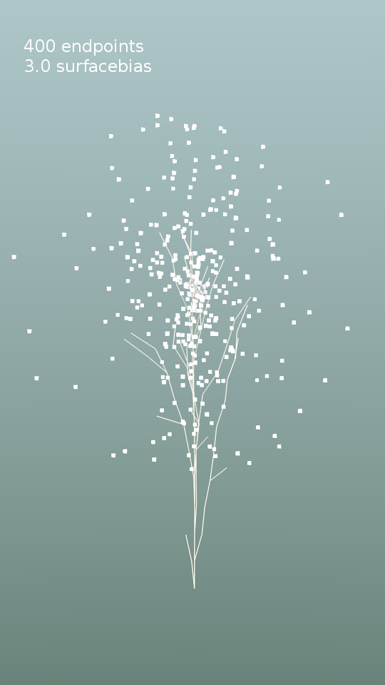
Near central axis vs. near surface
More endpoints near the top
Mix and match
Even shrubs are possible as shown on the right.
adding leaves
When you click the add leaves button a new panel with options will appear with controls for the leaves. The number of leaves controls the probability that an internode (branch segment) carries a leaf. The size and size variation of these leaves can be controlled, as well as the variation in orientation of the leaves. The number of connections option controls how much 'old wood' carries leaves. If you set this to 1 only new twigs will carry leaves.
Shaping the branches
When you click on the add modifiers option, three modifiers are added to the trunk skeleton (shown in the opening image of this article):
a subsurface modifier to smooth the branches,
a skin modifier to give volume to the branches and
another subsurface modifier to smooth this skin.
Note that calculating these last two modifiers may take many seconds or even minutes if the tree is complex! The thickness of the trunk and branches and the way the thickness of forking branches is combined is controlled by the Scale and Power options respectively.
Environmental influence
A final feature of this add-on that almost comes naturally with the space colonization algorithm is the ability to factor in environmental influences. For example if one side of the growing tree receives more shadow than the other side due to a wall or building, that side will grow less. We can easily mimick this by not placing any markers in a shadowed area. To accomplish this the add-on checks whether any of the markers is generates is inside any of the selected mesh objects in the scene and discards them if they are. The workflow is then:
select one or more objects (first image below)
position the 3d cursor where you want the tree to start
tweak any options
update the tree
The result (with markers) is shown in the second image below.
Note that we did not select the actual wall, but a larger duplicate (that we will not render), because the shadow influence normally extends beyond the wall and because a new branch might still pass through this exclusion zone towards markers that are above it. By chosing a wider volume we prevent those branches to pass through the actual wall.
Limitations
In this first version there will undoubtably be any number of bugs. One of the most annoying issues is that when the kill distance is chosen too small, a developing branch may terminate in a myriad of tiny segments. This will not only take an enormous amount of time when adding the skin modifier but will also cause a strange clump of hundreds of leaves at that point. Another thing is that even when not actually generating new geometry, the user interface is sometimes slow when modifiers are selected. I have a hunch this might be related to Blender keeping track of this complicated geometry in its undo cache but I am not sure. Of course there is also plenty of room for functional improvements: it would be nice if you could select more than one starting point for example to create hedgerows etc. and also have arbitrary objects instead of square leaves, but those are nice to haves for the future.
Some more examples
The following images show the same type of tree as the opening image of this article, but at more mature stages: The masked leaf texture as well as the concrete and brick textures are from cgtextures.com, the latter two converted to various types of specular and bump maps with the free shadermap commandline tool. The hdri-background is Alex Hart's 'Arboretrum in Bloom'. The most mature tree was generated with the settings shown below:
The advection vector doesn't have to be a constant: with some tweaking we can localize must of the vorticity to a single point on the sphre
Determining the distance to a point
The flow noise presented in a previous article has an advection parameter that determines how much small details are swept along with turbulent larger features. There is however nothing that prevents us to make this parameter dependent on the distance to some location to introduce some variation in the overall swirl patterns on the the sphere. An example is shown in the next video sample where the vorticity has its maximum near a point on the lower right front side:
Example node setup
The node setup looks like this:
The nodes in the yellow box calculate the distance to some hotspot ([1, -0.3, 1] not visible in this screenshot) and then calculate the lenght of this vector by determining the inproduct with itself. Then we add one to prevent division by zero in the next step, where we calculate the inverse. By raising it to some power we can control the 'tightness' of the spot, i.e. how fast our value decreases when we are further away from the hotspot. The final multiply node gives us some control on how strong the overall effect is.
In this article I present an OSL implementation of flow noise, both in 2D and in 4D
Flow Noise
in two previous posts (I, II) I showed a port to OSL of Stefan Gustavsons implementations of Simplex Noise and a fBM variant. Four dimensional Simplex Noise may be used to simulate the time evolution of 3D noise and in some situations like for example boiling liquids the result might be perfectly adequate. However if we want to capture the effects of swirls as seen in flowing liquids and gasses a better option is to use flow noise.
Flow noise was pioneered by Perlin and Neyret and the concept of adding vorticity (swirls) by rotating the lattice gradient vectors used to create the noise and adding higher octaves of noise at positions displaced by the lower octaves (advection) isn't limited to Perlin noise but can be applied to any lattice gradient noise, including Simplex Noise.
The code presented below is a straightforward and unoptimised port of Stefan Gustavsons original implementation in C. 2D and 3D versions of this noise are provided in a single shader,the type can be selected with the Dim parameter. By keyframing the Angle parameter you can create a swirling motion. The character of this motion may be influenced by altering the Octaves, lacunarity, H and advection parameters. The advection parameter basically determines how much small details in the flow will be swept along by the larger features.
Example node setup
The video of the swirling sphere was created with the following node setup:
The angle parameter was varied from 0 to 6.28 in 150 frames.
An additional trick to restrict the advection to some specific point is illustrated in another post.
The shader is an unwieldy large piece of code but nevertheless presented here in its entirety. Just click view plain to download it.
/* Simplex flow noise in 2 and 3D
 *
 * Based on Stefan Gustavsons orignal implementation in srdnoise23.c
 * (http://webstaff.itn.liu.se/~stegu/simplexnoise/DSOnoises.html)
 *
 * OSL port Michel Anders (varkenvarken) 2013-02-04
 * original comment is is left mostly in place, OSL specific comments
 * are preceded by MJA
 *
 * This code was placed in the public domain by its original author,
 * Stefan Gustavson. You may use it as you see fit, but
 * attribution is appreciated.
 *
*/
int FASTFLOOR(float x) {
 int xi = (int)x;
 return x < xi ? xi-1 : xi;
}

shader flownoise(
 point Pos = P,
 float Scale = 1,
 int Octaves = 1,
 float H = 1,
 float lacunarity=2,
 float Angle=0,
 float advection=0,
 int Dim = 2,
 output float fac = 0
){
 int perm[512] = {151,160,137,91,90,15,
 131,13,201,95,96,53,194,233,7,225,140,36,103,30,69,142,8,99,37,240,21,10,23,
 190, 6,148,247,120,234,75,0,26,197,62,94,252,219,203,117,35,11,32,57,177,33,
 88,237,149,56,87,174,20,125,136,171,168, 68,175,74,165,71,134,139,48,27,166,
 77,146,158,231,83,111,229,122,60,211,133,230,220,105,92,41,55,46,245,40,244,
 102,143,54, 65,25,63,161, 1,216,80,73,209,76,132,187,208, 89,18,169,200,196,
 135,130,116,188,159,86,164,100,109,198,173,186, 3,64,52,217,226,250,124,123,
 5,202,38,147,118,126,255,82,85,212,207,206,59,227,47,16,58,17,182,189,28,42,
 223,183,170,213,119,248,152, 2,44,154,163, 70,221,153,101,155,167, 43,172,9,
 129,22,39,253, 19,98,108,110,79,113,224,232,178,185, 112,104,218,246,97,228,
 251,34,242,193,238,210,144,12,191,179,162,241, 81,51,145,235,249,14,239,107,
 49,192,214, 31,181,199,106,157,184, 84,204,176,115,121,50,45,127, 4,150,254,
 138,236,205,93,222,114,67,29,24,72,243,141,128,195,78,66,215,61,156,180,
 151,160,137,91,90,15,
 131,13,201,95,96,53,194,233,7,225,140,36,103,30,69,142,8,99,37,240,21,10,23,
 190, 6,148,247,120,234,75,0,26,197,62,94,252,219,203,117,35,11,32,57,177,33,
 88,237,149,56,87,174,20,125,136,171,168, 68,175,74,165,71,134,139,48,27,166,
 77,146,158,231,83,111,229,122,60,211,133,230,220,105,92,41,55,46,245,40,244,
 102,143,54, 65,25,63,161, 1,216,80,73,209,76,132,187,208, 89,18,169,200,196,
 135,130,116,188,159,86,164,100,109,198,173,186, 3,64,52,217,226,250,124,123,
 5,202,38,147,118,126,255,82,85,212,207,206,59,227,47,16,58,17,182,189,28,42,
 223,183,170,213,119,248,152, 2,44,154,163, 70,221,153,101,155,167, 43,172,9,
 129,22,39,253, 19,98,108,110,79,113,224,232,178,185, 112,104,218,246,97,228,
 251,34,242,193,238,210,144,12,191,179,162,241, 81,51,145,235,249,14,239,107,
 49,192,214, 31,181,199,106,157,184, 84,204,176,115,121,50,45,127, 4,150,254,
 138,236,205,93,222,114,67,29,24,72,243,141,128,195,78,66,215,61,156,180};
 // MJA precomputing this table instead of calculating it as done in the
 // original code saves 30% running time.
 int permMod12[512] = { 7, 4, 5, 7, 6, 3, 11, 1, 9, 11, 0, 5, 2, 5, 7, 9, 8,
 0, 7, 6, 9, 10, 8, 3, 1, 0, 9, 10, 11, 10, 6, 4, 7, 0, 6, 3, 0, 2, 5, 2, 10,
 0, 3, 11, 9, 11, 11, 8, 9, 9, 9, 4, 9, 5, 8, 3, 6, 8, 5, 4, 3, 0, 8, 7, 2, 9,
 11, 2, 7, 0, 3, 10, 5, 2, 2, 3, 11, 3, 1, 2, 0, 7, 1, 2, 4, 9, 8, 5, 7, 10,
 5, 4, 4, 6, 11, 6, 5, 1, 3, 5, 1, 0, 8, 1, 5, 4, 0, 7, 4, 5, 6, 1, 8, 4, 3,
 10, 8, 8, 3, 2, 8, 4, 1, 6, 5, 6, 3, 4, 4, 1, 10, 10, 4, 3, 5, 10, 2, 3, 10,
 6, 3, 10, 1, 8, 3, 2, 11, 11, 11, 4, 10, 5, 2, 9, 4, 6, 7, 3, 2, 9, 11, 8, 8,
 2, 8, 10, 7, 10, 5, 9, 5, 11, 11, 7, 4, 9, 9, 10, 3, 1, 7, 2, 0, 2, 7, 5, 8,
 4, 10, 5, 4, 8, 2, 6, 1, 0, 11, 10, 2, 1, 10, 6, 0, 0, 11, 11, 6, 1, 9, 3, 1,
 7, 9, 2, 11, 11, 1, 0, 10, 7, 1, 7, 10, 1, 4, 0, 0, 8, 7, 1, 2, 9, 7, 4, 6, 2,
 6, 8, 1, 9, 6, 6, 7, 5, 0, 0, 3, 9, 8, 3, 6, 6, 11, 1, 0, 0, 7, 4, 5, 7, 6, 3,
 11, 1, 9, 11, 0, 5, 2, 5, 7, 9, 8, 0, 7, 6, 9, 10, 8, 3, 1, 0, 9, 10, 11, 10,
 6, 4, 7, 0, 6, 3, 0, 2, 5, 2, 10, 0, 3, 11, 9, 11, 11, 8, 9, 9, 9, 4, 9, 5, 8,
 3, 6, 8, 5, 4, 3, 0, 8, 7, 2, 9, 11, 2, 7, 0, 3, 10, 5, 2, 2, 3, 11, 3, 1, 2,
 0, 7, 1, 2, 4, 9, 8, 5, 7, 10, 5, 4, 4, 6, 11, 6, 5, 1, 3, 5, 1, 0, 8, 1, 5, 4,
 0, 7, 4, 5, 6, 1, 8, 4, 3, 10, 8, 8, 3, 2, 8, 4, 1, 6, 5, 6, 3, 4, 4, 1, 10, 10,
 4, 3, 5, 10, 2, 3, 10, 6, 3, 10, 1, 8, 3, 2, 11, 11, 11, 4, 10, 5, 2, 9, 4, 6, 7,
 3, 2, 9, 11, 8, 8, 2, 8, 10, 7, 10, 5, 9, 5, 11, 11, 7, 4, 9, 9, 10, 3, 1, 7, 2,
 0, 2, 7, 5, 8, 4, 10, 5, 4, 8, 2, 6, 1, 0, 11, 10, 2, 1, 10, 6, 0, 0, 11, 11, 6,
 1, 9, 3, 1, 7, 9, 2, 11, 11, 1, 0, 10, 7, 1, 7, 10, 1, 4, 0, 0, 8, 7, 1, 2, 9, 7,
 4, 6, 2, 6, 8, 1, 9, 6, 6, 7, 5, 0, 0, 3, 9, 8, 3, 6, 6, 11, 1, 0, 0};

 /*
  * Gradient tables. These could be programmed the Ken Perlin way with
  * some clever bit-twiddling, but this is more clear, and not really slower.
  */
 vector grad2[8] = {
   vector( -1.0, -1.0 , 0.0), vector( 1.0, 0.0 , 0.0) , vector( -1.0, 0.0 , 0.0) , vector( 1.0, 1.0 , 0.0) ,
   vector( -1.0, 1.0 , 0.0) , vector( 0.0, -1.0 , 0.0) , vector( 0.0, 1.0 , 0.0) , vector( 1.0, -1.0 , 0.0)
 };

 /*
  * For 3D, we define two orthogonal vectors in the desired rotation plane.
  * These vectors are based on the midpoints of the 12 edges of a cube,
  * they all rotate in their own plane and are never coincident or collinear.
  * A larger array of random vectors would also do the job, but these 12
  * (including 4 repeats to make the array length a power of two) work better.
  * They are not random, they are carefully chosen to represent a small
  * isotropic set of directions for any rotation angle.
  */

 /* a = sqrt(2)/sqrt(3) = 0.816496580 */
#define a 0.81649658

 vector grad3u[16] = {
   vector( 1.0, 0.0, 1.0 ), vector( 0.0, 1.0, 1.0 ), // 12 cube edges
   vector( -1.0, 0.0, 1.0 ), vector( 0.0, -1.0, 1.0 ),
   vector( 1.0, 0.0, -1.0 ), vector( 0.0, 1.0, -1.0 ),
   vector( -1.0, 0.0, -1.0 ), vector( 0.0, -1.0, -1.0 ),
   vector( a, a, a ), vector( -a, a, -a ),
   vector( -a, -a, a ), vector( a, -a, -a ),
   vector( -a, a, a ), vector( a, -a, a ),
   vector( a, -a, -a ), vector( -a, a, -a )
 };

 vector grad3v[16] = {
   vector( -a, a, a ), vector( -a, -a, a ),
   vector( a, -a, a ), vector( a, a, a ),
   vector( -a, -a, -a ), vector( a, -a, -a ),
   vector( a, a, -a ), vector( -a, a, -a ),
   vector( 1.0, -1.0, 0.0 ), vector( 1.0, 1.0, 0.0 ),
   vector( -1.0, 1.0, 0.0 ), vector( -1.0, -1.0, 0.0 ),
   vector( 1.0, 0.0, 1.0 ), vector( -1.0, 0.0, 1.0 ), // 4 repeats to make 16
   vector( 0.0, 1.0, -1.0 ), vector( 0.0, -1.0, -1.0 )
 };

#undef a

 /*
  * Helper functions to compute rotated gradients and
  * gradients-dot-residualvectors in 2D and 3D.
  */

 void gradrot2( int hash, float sin_t, float cos_t, float gx, float gy ) {
  int h = hash & 7;
  float gx0 = grad2[h][0];
  float gy0 = grad2[h][1];
  gx = cos_t * gx0 - sin_t * gy0;
  gy = sin_t * gx0 + cos_t * gy0;
  return;
 }

 void gradrot3( int hash, float sin_t, float cos_t, float gx, float gy, float gz ) {
  int h = hash & 15;
  float gux = grad3u[h][0];
  float guy = grad3u[h][1];
  float guz = grad3u[h][2];
  float gvx = grad3v[h][0];
  float gvy = grad3v[h][1];
  float gvz = grad3v[h][2];
  gx = cos_t * gux + sin_t * gvx;
  gy = cos_t * guy + sin_t * gvy;
  gz = cos_t * guz + sin_t * gvz;
  return;
 }

 float graddotp3( float gx, float gy, float gz, float x, float y, float z ) {
  return gx * x + gy * y + gz * z;
 }

 float angle = Angle; // MJA copy input parameter so that we can write it

 float pwr = 1.0;
 float pwHL = pow(lacunarity,-H);

 /* Skewing factors for 2D simplex grid:
  * F2 = 0.5*(sqrt(3.0)-1.0)
  * G2 = (3.0-Math.sqrt(3.0))/6.0
  */
#define F2 0.366025403
#define G2 0.211324865

 /** 2D simplex noise with derivatives.
  * If the last two arguments are not null, the analytic derivative
  * (the 2D gradient of the scalar noise field) is also calculated.
  */
 if( Dim == 2 ){
  float x = Pos[0]*Scale;
  float y = Pos[1]*Scale;
  float dnoise_dx;
  float dnoise_dy;
  float sin_t, cos_t; /* Sine and cosine for the gradient rotation angle */
  sin_t = sin( angle );
  cos_t = cos( angle );
  for(int p=0; p < Octaves; p++){
   float n0, n1, n2; /* Noise contributions from the three simplex corners */
   float gx0, gy0, gx1, gy1, gx2, gy2; /* Gradients at simplex corners */

   /* Skew the input space to determine which simplex cell we're in */
   float s = ( x + y ) * F2; /* Hairy factor for 2D */
   float xs = x + s;
   float ys = y + s;
   int i = FASTFLOOR( xs );
   int j = FASTFLOOR( ys );

   float t = ( i + j ) * G2;
   float X0 = i - t; /* Unskew the cell origin back to (x,y) space */
   float Y0 = j - t;
   float x0 = x - X0; /* The x,y distances from the cell origin */
   float y0 = y - Y0;

   /* For the 2D case, the simplex shape is an equilateral triangle.
    * Determine which simplex we are in. */
   int i1, j1; /* Offsets for second (middle) corner of simplex in (i,j) coords */
   if( x0 > y0 ) { i1 = 1; j1 = 0; } /* lower triangle, XY order: (0,0)->(1,0)->(1,1) */
   else { i1 = 0; j1 = 1; }      /* upper triangle, YX order: (0,0)->(0,1)->(1,1) */

   /* A step of (1,0) in (i,j) means a step of (1-c,-c) in (x,y), and
    * a step of (0,1) in (i,j) means a step of (-c,1-c) in (x,y), where
    * c = (3-sqrt(3))/6   */
   float x1 = x0 - i1 + G2; /* Offsets for middle corner in (x,y) unskewed coords */
   float y1 = y0 - j1 + G2;
   float x2 = x0 - 1.0 + 2.0 * G2; /* Offsets for last corner in (x,y) unskewed coords */
   float y2 = y0 - 1.0 + 2.0 * G2;

   /* Wrap the integer indices at 256, to avoid indexing perm[] out of bounds */
   int ii = i & 255; // MJA was % 256 but OSL mod is not the same as C %
   int jj = j & 255;

   /* Calculate the contribution from the three corners */
   float t0 = 0.5 - x0 * x0 - y0 * y0;
   float t20, t40;
   if( t0 < 0.0 ) t40 = t20 = t0 = n0 = gx0 = gy0 = 0.0; /* No influence */
   else {
     gradrot2( perm[ii + perm[jj]], sin_t, cos_t, gx0, gy0 );
     t20 = t0 * t0;
     t40 = t20 * t20;
     n0 = t40 * ( gx0 * x0 + gy0 * y0 );
   }

   float t1 = 0.5 - x1 * x1 - y1 * y1;
   float t21, t41;
   if( t1 < 0.0 ) t21 = t41 = t1 = n1 = gx1 = gy1 = 0.0; /* No influence */
   else {
     gradrot2( perm[ii + i1 + perm[jj + j1]], sin_t, cos_t, gx1, gy1 );
     t21 = t1 * t1;
     t41 = t21 * t21;
     n1 = t41 * ( gx1 * x1 + gy1 * y1 );
   }

   float t2 = 0.5 - x2 * x2 - y2 * y2;
   float t22, t42;
   if( t2 < 0.0 ) t42 = t22 = t2 = n2 = gx2 = gy2 = 0.0; /* No influence */
   else {
     gradrot2( perm[ii + 1 + perm[jj + 1]], sin_t, cos_t, gx2, gy2 );
     t22 = t2 * t2;
     t42 = t22 * t22;
     n2 = t42 * ( gx2 * x2 + gy2 * y2 );
   }

   /* Add contributions from each corner to get the final noise value.
    * The result is scaled to return values in the interval [-1,1]. */
   float noise = 70.0 * ( n0 + n1 + n2 ); // MJA scale factor was 40

   /* Compute derivative, if requested by supplying non-null pointers
    * for the last two arguments */
   if( advection != 0 ){
   /*  A straight, unoptimised calculation would be like:
    *    *dnoise_dx = -8.0 * t20 * t0 * x0 * ( gx0 * x0 + gy0 * y0 ) + t40 * gx0;
    *    *dnoise_dy = -8.0 * t20 * t0 * y0 * ( gx0 * x0 + gy0 * y0 ) + t40 * gy0;
    *    *dnoise_dx += -8.0 * t21 * t1 * x1 * ( gx1 * x1 + gy1 * y1 ) + t41 * gx1;
    *    *dnoise_dy += -8.0 * t21 * t1 * y1 * ( gx1 * x1 + gy1 * y1 ) + t41 * gy1;
    *    *dnoise_dx += -8.0 * t22 * t2 * x2 * ( gx2 * x2 + gy2 * y2 ) + t42 * gx2;
    *    *dnoise_dy += -8.0 * t22 * t2 * y2 * ( gx2 * x2 + gy2 * y2 ) + t42 * gy2;
    */
    float temp0 = t20 * t0 * ( gx0* x0 + gy0 * y0 );
    dnoise_dx = temp0 * x0;
    dnoise_dy = temp0 * y0;
    float temp1 = t21 * t1 * ( gx1 * x1 + gy1 * y1 );
    dnoise_dx += temp1 * x1;
    dnoise_dy += temp1 * y1;
    float temp2 = t22 * t2 * ( gx2* x2 + gy2 * y2 );
    dnoise_dx += temp2 * x2;
    dnoise_dy += temp2 * y2;
    dnoise_dx *= -8.0;
    dnoise_dy *= -8.0;
    dnoise_dx += t40 * gx0 + t41 * gx1 + t42 * gx2;
    dnoise_dy += t40 * gy0 + t41 * gy1 + t42 * gy2;
    dnoise_dx *= 70.0; /* Scale derivative to match the noise scaling */ // MJA scale factor was 40
    dnoise_dy *= 70.0;

    float advect_x = -advection * dnoise_dx;
    float advect_y = -advection * dnoise_dy;
    fac += noise * pwr;

    pwr *= pwHL;
    x *= lacunarity;
    y *= lacunarity;

    x += advect_x*pow(lacunarity,p);
    y += advect_y*pow(lacunarity,p);
    angle *= lacunarity;
   }else{
    fac += noise * pwr;
    pwr *= pwHL;
    x *= lacunarity;
    y *= lacunarity;
   }
  }
 }else if(Dim==3){
 /* Skewing factors for 3D simplex grid:
  * F3 = 1/3
  * G3 = 1/6 */
#define F3 0.333333333
#define G3 0.166666667

  float x=Pos[0]*Scale;
  float y=Pos[1]*Scale;
  float z=Pos[2]*Scale;
        float dnoise_dx;
  float dnoise_dy;
  float dnoise_dz;

  float n0, n1, n2, n3; /* Noise contributions from the four simplex corners */
  float noise;          /* Return value */
  float gx0, gy0, gz0, gx1, gy1, gz1; /* Gradients at simplex corners */
  float gx2, gy2, gz2, gx3, gy3, gz3;
  float sin_t, cos_t; /* Sine and cosine for the gradient rotation angle */
  sin_t = sin( angle );
  cos_t = cos( angle );
  for(int p=0; p < Octaves; p++){
   /* Skew the input space to determine which simplex cell we're in */
   float s = (x+y+z)*F3; /* Very nice and simple skew factor for 3D */
   float xs = x+s;
   float ys = y+s;
   float zs = z+s;
   int i = FASTFLOOR(xs);
   int j = FASTFLOOR(ys);
   int k = FASTFLOOR(zs);

   float t = (float)(i+j+k)*G3;
   float X0 = i-t; /* Unskew the cell origin back to (x,y,z) space */
   float Y0 = j-t;
   float Z0 = k-t;
   float x0 = x-X0; /* The x,y,z distances from the cell origin */
   float y0 = y-Y0;
   float z0 = z-Z0;

   /* For the 3D case, the simplex shape is a slightly irregular tetrahedron.
    * Determine which simplex we are in. */
   int i1, j1, k1; /* Offsets for second corner of simplex in (i,j,k) coords */
   int i2, j2, k2; /* Offsets for third corner of simplex in (i,j,k) coords */

   /* TODO: This code would benefit from a backport from the GLSL version! */
   if(x0>=y0) {
     if(y0>=z0)
    { i1=1; j1=0; k1=0; i2=1; j2=1; k2=0; } /* X Y Z order */
    else if(x0>=z0) { i1=1; j1=0; k1=0; i2=1; j2=0; k2=1; } /* X Z Y order */
    else { i1=0; j1=0; k1=1; i2=1; j2=0; k2=1; } /* Z X Y order */
     }
   else { // x0 < y0
     if(y0 < z0) { i1=0; j1=0; k1=1; i2=0; j2=1; k2=1; } /* Z Y X order */
     else if(x0 < z0) { i1=0; j1=1; k1=0; i2=0; j2=1; k2=1; } /* Y Z X order */
     else { i1=0; j1=1; k1=0; i2=1; j2=1; k2=0; } /* Y X Z order */
   }

   /* A step of (1,0,0) in (i,j,k) means a step of (1-c,-c,-c) in (x,y,z),
    * a step of (0,1,0) in (i,j,k) means a step of (-c,1-c,-c) in (x,y,z), and
    * a step of (0,0,1) in (i,j,k) means a step of (-c,-c,1-c) in (x,y,z), where
    * c = 1/6.   */

   float x1 = x0 - i1 + G3; /* Offsets for second corner in (x,y,z) coords */
   float y1 = y0 - j1 + G3;
   float z1 = z0 - k1 + G3;
   float x2 = x0 - i2 + 2.0 * G3; /* Offsets for third corner in (x,y,z) coords */
   float y2 = y0 - j2 + 2.0 * G3;
   float z2 = z0 - k2 + 2.0 * G3;
   float x3 = x0 - 1.0 + 3.0 * G3; /* Offsets for last corner in (x,y,z) coords */
   float y3 = y0 - 1.0 + 3.0 * G3;
   float z3 = z0 - 1.0 + 3.0 * G3;

   /* Wrap the integer indices at 256, to avoid indexing perm[] out of bounds */
   int ii = i & 255; // MJA was % 256 but OSL mod is not the same as C %
   int jj = j & 255;
   int kk = k & 255;

   /* Calculate the contribution from the four corners */
   float t0 = 0.6 - x0*x0 - y0*y0 - z0*z0;
   float t20, t40;
   if(t0 < 0.0) n0 = t0 = t20 = t40 = gx0 = gy0 = gz0 = 0.0;
   else {
     gradrot3( perm[ii + perm[jj + perm[kk]]], sin_t, cos_t, gx0, gy0, gz0 );
     t20 = t0 * t0;
     t40 = t20 * t20;
     n0 = t40 * graddotp3( gx0, gy0, gz0, x0, y0, z0 );
   }

   float t1 = 0.6 - x1*x1 - y1*y1 - z1*z1;
   float t21, t41;
   if(t1 < 0.0) n1 = t1 = t21 = t41 = gx1 = gy1 = gz1 = 0.0;
   else {
     gradrot3( perm[ii + i1 + perm[jj + j1 + perm[kk + k1]]], sin_t, cos_t, gx1, gy1, gz1 );
     t21 = t1 * t1;
     t41 = t21 * t21;
     n1 = t41 * graddotp3( gx1, gy1, gz1, x1, y1, z1 );
   }

   float t2 = 0.6 - x2*x2 - y2*y2 - z2*z2;
   float t22, t42;
   if(t2 < 0.0) n2 = t2 = t22 = t42 = gx2 = gy2 = gz2 = 0.0;
   else {
     gradrot3( perm[ii + i2 + perm[jj + j2 + perm[kk + k2]]], sin_t, cos_t, gx2, gy2, gz2 );
     t22 = t2 * t2;
     t42 = t22 * t22;
     n2 = t42 * graddotp3( gx2, gy2, gz2, x2, y2, z2 );
   }

   float t3 = 0.6 - x3*x3 - y3*y3 - z3*z3;
   float t23, t43;
   if(t3 < 0.0) n3 = t3 = t23 = t43 = gx3 = gy3 = gz3 = 0.0;
   else {
     gradrot3( perm[ii + 1 + perm[jj + 1 + perm[kk + 1]]], sin_t, cos_t, gx3, gy3, gz3 );
     t23 = t3 * t3;
     t43 = t23 * t23;
     n3 = t43 * graddotp3( gx3, gy3, gz3, x3, y3, z3 );
   }

   /*  Add contributions from each corner to get the final noise value.
    * The result is scaled to return values in the range [-1,1] */
   noise = 28.0 * (n0 + n1 + n2 + n3);

   /* Compute derivative, if requested by supplying non-null pointers
    * for the last three arguments */
   if(advection != 0){
   /*  A straight, unoptimised calculation would be like:
    *     *dnoise_dx = -8.0f * t20 * t0 * x0 * graddotp3(gx0, gy0, gz0, x0, y0, z0) + t40 * gx0;
    *    *dnoise_dy = -8.0f * t20 * t0 * y0 * graddotp3(gx0, gy0, gz0, x0, y0, z0) + t40 * gy0;
    *    *dnoise_dz = -8.0f * t20 * t0 * z0 * graddotp3(gx0, gy0, gz0, x0, y0, z0) + t40 * gz0;
    *    *dnoise_dx += -8.0f * t21 * t1 * x1 * graddotp3(gx1, gy1, gz1, x1, y1, z1) + t41 * gx1;
    *    *dnoise_dy += -8.0f * t21 * t1 * y1 * graddotp3(gx1, gy1, gz1, x1, y1, z1) + t41 * gy1;
    *    *dnoise_dz += -8.0f * t21 * t1 * z1 * graddotp3(gx1, gy1, gz1, x1, y1, z1) + t41 * gz1;
    *    *dnoise_dx += -8.0f * t22 * t2 * x2 * graddotp3(gx2, gy2, gz2, x2, y2, z2) + t42 * gx2;
    *    *dnoise_dy += -8.0f * t22 * t2 * y2 * graddotp3(gx2, gy2, gz2, x2, y2, z2) + t42 * gy2;
    *    *dnoise_dz += -8.0f * t22 * t2 * z2 * graddotp3(gx2, gy2, gz2, x2, y2, z2) + t42 * gz2;
    *    *dnoise_dx += -8.0f * t23 * t3 * x3 * graddotp3(gx3, gy3, gz3, x3, y3, z3) + t43 * gx3;
    *    *dnoise_dy += -8.0f * t23 * t3 * y3 * graddotp3(gx3, gy3, gz3, x3, y3, z3) + t43 * gy3;
    *    *dnoise_dz += -8.0f * t23 * t3 * z3 * graddotp3(gx3, gy3, gz3, x3, y3, z3) + t43 * gz3;
    */
    float temp0 = t20 * t0 * graddotp3( gx0, gy0, gz0, x0, y0, z0 );
    dnoise_dx = temp0 * x0;
    dnoise_dy = temp0 * y0;
    dnoise_dz = temp0 * z0;
    float temp1 = t21 * t1 * graddotp3( gx1, gy1, gz1, x1, y1, z1 );
    dnoise_dx += temp1 * x1;
    dnoise_dy += temp1 * y1;
    dnoise_dz += temp1 * z1;
    float temp2 = t22 * t2 * graddotp3( gx2, gy2, gz2, x2, y2, z2 );
    dnoise_dx += temp2 * x2;
    dnoise_dy += temp2 * y2;
    dnoise_dz += temp2 * z2;
    float temp3 = t23 * t3 * graddotp3( gx3, gy3, gz3, x3, y3, z3 );
    dnoise_dx += temp3 * x3;
    dnoise_dy += temp3 * y3;
    dnoise_dz += temp3 * z3;
    dnoise_dx *= -8.0;
    dnoise_dy *= -8.0;
    dnoise_dz *= -8.0;
    /* This corrects a bug in the original implementation */
    dnoise_dx += t40 * gx0 + t41 * gx1 + t42 * gx2 + t43 * gx3;
    dnoise_dy += t40 * gy0 + t41 * gy1 + t42 * gy2 + t43 * gy3;
    dnoise_dz += t40 * gz0 + t41 * gz1 + t42 * gz2 + t43 * gz3;
    dnoise_dx *= 28.0; /* Scale derivative to match the noise scaling */
    dnoise_dy *= 28.0;
    dnoise_dz *= 28.0;

    float advect_x = -advection * dnoise_dx;
    float advect_y = -advection * dnoise_dy;
    float advect_z = -advection * dnoise_dz;
    fac += noise * pwr;

    pwr *= pwHL;
    x *= lacunarity;
    y *= lacunarity;

    x += advect_x*pow(lacunarity,p);
    y += advect_y*pow(lacunarity,p);
    y += advect_z*pow(lacunarity,p);
    angle *= lacunarity;
   }else{
    fac += noise * pwr;
    pwr *= pwHL;
    x *= lacunarity;
    y *= lacunarity;
    z *= lacunarity;
   }
  }
 }
}
 The new skinning method is the default if you uncheck the no modifiers checkbox but if you like you can still select Blenders skin modifier from the drop down as shown on the right. (This can also be done later because we leave the skeleton itself intact; as it only consists of edges it won't show up in renders but you could use it to add any modifier later on).
  When we apply a subsurface modifier to our skinned branches the result is already quite acceptable although I see room for improvement, specifically in the shape of the forks. As you can see there is some bulging were the branches join and this is especially noticeable when there is either a very sharp anngle between the branches or when both branches bend out of plane. Fortunately the highlighted 5-gon lends itself to all kinds of angle dependant adaptations so I expect I can tweak this further to get smoother results.