This is an article in a multipart series on the concepts of ray tracing. I am not sure where this will lead but I am open to suggestions. We will be creating code that will run inside Blender. Blender has ray tracing renderers of course but that is not the point: by reusing Python libraries and Blender's scene building capabilities we can concentrate on true ray tracing issues like shader models, lighting, etc.
I generally present stuff in a back-to-front manner: first an article with some (well commented) code and images of the results, then one or more articles discussing the concepts. The idea is that this encourages you to experiment and have a look at the code yourself before being introduced to theory. How well this works out we will see :-)
So far the series consists of the several articles labeled
ray tracing concepts
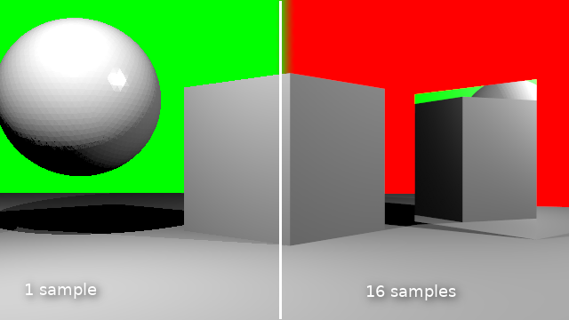
Anti aliasing
If we want to diminish the jagged look of edges in our rendered image we can sample a pixel multiple times at slightly different positions and average the result. In this article I show the code to do this.
Code
Once we know how many times we want to sample a pixel we have to calculate our camera ray as many times but with slightly shifted coordinates and then average the result. If we take the original direction of the camera ray to point into the exact middle of an on screen pixel, we have pick a point in the square centered around this point.
For this we first calculate the size of this square (line 9 and 10). Then as before we calculate each pixel but we repeat this for every sample (line 14). We keep the sum of all our samples in a separate buffer
sbuf (defined in line 5, the addition is in line 23). We still want the final buffer that will be shown on screen to represent the averaged color we calculated so far, so in line 15 we update a whole line of pixels to represent the current average.
We also invert the line above it (line 16,17) so we have some visual feedback of where we are when we are updating the buffer. This is useful to keep track as with increasing samples the contribition gets smaller and might be hardto see.
Finally we yield the percentage of samples we calculated so far.
Note that the
vdc() function returns a number from a Van der Corput sequence. I have not shown this function and you could use uniformly distributed random numbers instead (shown in the line that is commented out) in stead of these quasi random numbers, but these should give better results. The reasoning behind this is out of scope of this article but
check Wikipedia for more on this.
def ray_trace(scene, width, height, depth, buf, samples, gi):

    ... indentical code left out ...

    sbuf = np.zeros(width*height*4)
    sbuf.shape = height,width,4

    aspectratio = height/width
    dy = aspectratio/height
    dx = 1/width
    seed(42)

    N = samples*width*height
    for s in range(samples):
        for y in range(height):
            yscreen = ((y-(height/2))/height) * aspectratio
            for x in range(width):
                xscreen = (x-(width/2))/width
                #dir = Vector((xscreen + dx*(random()-0.5), yscreen + dy*(random()-0.5), -1))
                dir = Vector((xscreen + dx*(vdc(s,2)-0.5), yscreen + dy*(vdc(s,3)-0.5), -1))
                dir.rotate(rotation)
                dir = dir.normalized()
                sbuf[y,x,0:3] += single_ray(scene, origin, dir, lamps, depth, gi)
            buf[y,:,0:3] = sbuf[y,:,0:3] / (s+1)
            if y < height-1:
                buf[y+1,:,0:3] = 1 - buf[y+1,:,0:3]
            yield (s*width*height+width*y)/N
When we call our new
ray_trace() function we have to determine the number of samples first. Blender provides two properties from the render context for this:
scene.render.use_antialiasing and
scene.render.antialiasing_samples. For some reason that last one is a string, so we have to convert it to an int before we can use it:
    def render_scene(self, scene):

    ... indentical code left out ...

        samples = int(scene.render.antialiasing_samples) if scene.render.use_antialiasing else 1
        for p in ray_trace(scene, width, height, 1, buf, samples, gi):

    ... indentical code left out ...
Now we could make the whole existing anti-aliasing panel available by again adding our engine to the
COMPAT_ENGINES attribute but because it had lots of options we don't use we create our own panel with just the properties we need (something we might do later for other panels as well):
from bpy.types import Panel
from bl_ui.properties_render import RenderButtonsPanel

class CUSTOM_RENDER_PT_antialiasing(RenderButtonsPanel, Panel):
    bl_label = "Anti-Aliasing"
    COMPAT_ENGINES = {CustomRenderEngine.bl_idname}

    def draw_header(self, context):
        rd = context.scene.render

        self.layout.prop(rd, "use_antialiasing", text="")

    def draw(self, context):
        layout = self.layout

        rd = context.scene.render
        layout.active = rd.use_antialiasing

        split = layout.split()

        col = split.column()
        col.row().prop(rd, "antialiasing_samples", expand=True)
Code availability
The revision containing the code changes from this article is
available from GitHub.