Face area to vertex color add-on, can we improve wireframe renders?
Blender procedural hexagon pattern
Availability
Implementation details
Extended Voronoi Texture support in Blender
But all of a sudden there has been some interest again and now we have extended Voronoi functionality in the Voronoi texture node! And of course Pablo in his unique enthusiastic style did a nice demo of it as well check out the video.
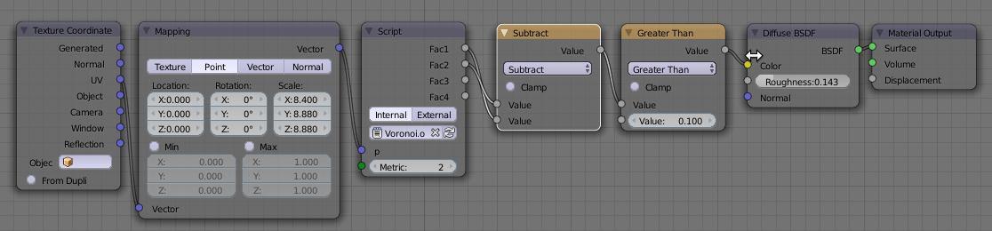
The new functionality is available in the latest build of 2.79 and presumably in the 2.8 branch too. Note that in my original patch I included Voronoi crackle as well, but that is not available in the new node itself. However since Voronoi crackle is simply the difference between the distance to the 2nd closest and the 1st closest point, this popular pattern is super easy to implement now with the following noodle:
Finally an easy way to generate lizard scales :-)
Approximating translucency with inverse ambient occlusion in Blender
The idea is simple enough: just create a map for each position at the inside of the mesh with a value that represents how much light would be received at that point from nearby surfaces. Sounds a lot like ambient occlusion so the idea is to use ambient occlusion baking but with the normals inverted. The only snag is that inside a mesh it is extremely unlikely that a ray will ever reach the sky (even impossible if the mesh is watertight), resulting in a black map. However, Blenders AO settings have a distance parameter that can be used to tell the AO baking that any ray that does not hit a surface within this distance is considered sky: 
(Note that we do not even have to enable AO for our purpose, i.e. baking, just setting the distance to 0.1 or something will suffice)
Now we can create a map that approximates translucency with the following steps:
- Invert the normals on the mesh (they should all point inward)
- Bake the ambient occlusion to an image texture (documented here)
- Make sure you point the normals to the outside again
- Use the inverted values of the image as a translucency map.

The noodle that uses this map to illustrate their values with an emission shader is shown below

Now if this is really useful to for example tweak a subsurface scattering shader is up to you :-) If you create a skin shader with it I am eager to see the results.
Extending the Voronoi node in Cycles: a progress report
Basically the Cycles Voronoi texture node will have all the functionality of its Blender Internal counterpart: you can choose different metrics (= ways to define what a distance is) including the manhattan and chebychev metrics and you can choose whether you want to closest neighbor, the 2nd closest (and 3rd, 4th) or the difference between the 2dn and the 1st closest (a.k.a. Voronoi Crackle). A sample is shown below: 
The node has the same outputs as before and just has two extra buttons and an extra input socket (E, which controls the exponent of the Minkovski metric): 
The node defaults to the old options and produces output that is pixel for pixel identical to the old output (with a distance metric of Distance squared). The downside of all this extra functionality is that it is slightly slower (because it now has to choose between different metrics and has to keep around more data). So currently I am checking if or where it makes sense to optimize the code some more. I don't want to complicate the code too much because that would make both maintaining and reviewing the code harder, so at this point it might be more sensible to let it be and accept a few percent penalty for now.
How to add a new node to the Cycles source code
The page is listed in the pages widget on the top right of the blog or via this link.
Hexagon shader texture for Blender Cycles on GPU and CPU

The image was created with the following noodle:

As you can see, the hexagon node provide both a color and two float outputs. The first is the distance squared to the centre of the hexagon, the second one the distance squared to the centre of the nearest neighbour. Having both output allows for the easy creation of an edge, as shown in the noodle.
Code
The code follows the implementation of the OSL version closely and might be sub-optimal. My first steps will be to document my steps in creating a completely new node (because no less than 15(!) files needed to be changed or added to implement a single node. After that I want to optimize the code a bit and wait for feedback on my previous patch before submitting this one.Voronoi playtime, redux
There still isn't but prompted by a question I decided to implement it in an ugly way; after all, if it works that is all that matters :-). All the necessary code to implement different distance metrics is already in node_texture.h but for some reason it was commented out. I therefore lifted the necessary part from this file and combined it with a a small shader that lets you choose the distance metric with an integer. An example for the Manhattan metric is shown below.
Node setup and code availability
The node setup used to generate the image above looks like this:
The code for the shader is available on GitHub. The node it generates may look a bit different than in the noodle shown here because I added an exponent input
E that can be used for the generalized Minkovsky metric (metric == 6). Using vertex colors to color hair in Cycles

For this image WeightLifter was used to create a vertex group with more weight on horizontal surface:

Then this vertex group was used to control the distribution of the hairs by selecting the gruop in the particle system settings:

In the same manner WeightLifter was used to create vertex colors that change colors from left to right:

A Cycles material was then created to use these vertex colors (via the Attribute node) to color the hairs
A hexagon shader in OSL, second edition

The noodle used to create the image is shown below (click to enlarge):

The color code has stayed the same except for the calculation of the distance to the edge. This might be a bit inefficient, but at least it's easy to read.
The additions are shown below, the full code is available on GitHub.
// distance to nearest edge
float x = mod(Coordinates[0]/3,1.0);
float y = mod(Coordinates[1]/3,A2);
#define N 18
vector hc[N] = {
vector( 0, -A2/3 ,0),
vector( 0, 0 ,0),
vector( 0, A2/3 ,0),
vector( 0,2*A2/3 ,0),
vector( 0, A2 ,0),
vector( 0,4*A2/3 ,0),
vector(0.5, -A2/3+A2/6,0),
vector(0.5, 0+A2/6,0),
vector(0.5, A2/3+A2/6,0),
vector(0.5,2*A2/3+A2/6,0),
vector(0.5, A2 +A2/6,0),
vector(0.5,4*A2/3+A2/6,0),
vector(1.0, -A2/3 ,0),
vector(1.0, 0 ,0),
vector(1.0, A2/3 ,0),
vector(1.0,2*A2/3 ,0),
vector(1.0, A2 ,0),
vector(1.0,4*A2/3 ,0)
};
float d[N], t;
for(int i=0; i < N; i++){
float dx = x - hc[i][0];
float dy = y - hc[i][1];
d[i] = hypot(dx, dy);
}
for(int j= N-1; j >= 0; j--){
for(int i= 0; i < j; i++){
if(d[i] > d[i+1]){
SWAP(t, d[i], d[i+1]);
}
}
}
Center = d[0];
Edge = d[1] - d[0];
InEdge = Edge < Width;
The approach we have taken is very simple: the hc enumerates all nearby hexagon centers. We then calculate all the distances to these points and sort them shortest to longest (yes with a bubble sort: with 18 elements it might just be faster to do it with a more efficient sorting algorithm at the cost of much more complex code so I don't bother). The
Edge is not realy the distance to the closest edge but the difference between the closest center and the next closest. Near the edge these values are more and more the same so Edge will approach zero. For convience we provide a comparison with some threshold also. A new tree addon, Part IV: volume rendering experiments with OSL

This effect was achieved by inserting a scaled icosphere that covers about 90% of the crown interior (see below) and adding a volume shader to this icosphere that scatters and absorbs light in a non-uniform manner, i.e. the shader mimics a bunch of small scattered disks, which when seen from the distance add to the illusion of leaves. Note that we cannot do without all the leaves because volume scattering adds no specular reflections as real leaves might do.

Shader code and example node setup
The code for this shader consists of the shader proper, which merely checks which randomly scattered point we are closest to and then calls theindisk function with the position of this closest point and a random direction. indisk checks whether we are inside a disk with its axis in some direction and returns 1 if this is indeed so. Note that the include at the start of the code refers to a file that is distriubted with Blender and contains a number of useful functions, including a number of Voronoi/Worley related ones.
#include "node_texture.h"
int indisk(
point p,
point c, float r, float h, vector d
){
vector v = p - c;
float a = dot(v,d);
float lh = abs(length(a * d));
if(lh > h){ return 0;}
float lv = length(v);
float lp = sqrt(lv*lv - lh*lh);
if(lp > r){ return 0;}
return 1;
}
vector randomdirection(point p){
float t = M_2PI*noise("cell",p,1);
float u = 2*noise("cell",p,2)-1;
float s,c,a;
sincos(t,s,c);
a = sqrt(1-u*u);
float x = a*c;
float y = a*s;
float z = u;
return vector(x,y,z);
}
shader bits(
point Pos = P,
float Scale = 1,
float Size = 1,
float Height = 0.05,
output float Fac = 0
){
point p = Pos * Scale;
point centers[4];
float distances[4];
voronoi(p, "Distance Squared", 0, distances, centers);
if(indisk(p,centers[0],Size,Height,randomdirection(p))){
Fac = 1;
}
}
The node setup to use this shader as seen in the opening image of this article looks like this:
Discussion
Whether using a volume shader this way is really useful remains to be seen: rendering this way is still rather slow. Of course, getting a comparable dense crown with extra particles also slows down rendering: in my tests doubling the number of particles from 1000 to 2000 resulted in a render time that was actually slower than adding the volume shader. In other words, your mileage may vary but it might be worth to experiment.References
The space tree addon itself is introduced in a few articles on this blog and is available on GitHub. Relevant links are listed below:Creating unique snowflakes with OSL
The shader presented in this article will create a unique snowflake for each value of its
Seed. Using the object info node we may obtain a unique random number for each object that we may use for this purpose as we will see when we examine the node setup. Snowflakes
The code below defines the following utility functions;- hex
- this function will produce the x and y coordinates of a point as it is rotated through the six segments of a hexagon
- in_hexagon
- this function will return a non zero value if a point lies within a hexagon
- pattern
- this function does the real work. It returns non zero if a point is positioned within a number of hexagons that are randomly positioned along the x-axis. It also draws a connecting rod that extends as far as the farthest hexagon.
pattern(). Note that because we expect uv-coordinates for a simple square (I.e in de range [0,1], we transform these coordinates so that the center is at (0.5, 0.5) [line 68].
#define SLOPE 1/sqrt(3)
#define SIDE sqrt(.75)
#define D60c cos(radians(60))
#define D60s sin(radians(60))
void hex(float x, float y, output float hx[6], output float hy[6]){
hx[0]=x;
hy[0]=y;
hx[1]=x*D60c-y*D60s;
hy[1]=y*D60c+x*D60s;
hx[2]=x*D60c+y*D60s;;
hy[2]=y*D60c-x*D60s;
hx[3]=-hx[0];
hy[3]=-hy[0];
hx[4]=-hx[1];
hy[4]=-hy[1];
hx[5]=-hx[2];
hy[5]=-hy[2];
}
int in_hexagon(
float px, float py,
float cx, float cy, float r,
output float d
){
d=hypot(px-cx,py-cy);
if(d>r){ return 0; }
float hx[6],hy[6];
hex(px-cx, py-cy, hx, hy);
for(int h=0; h < 6; h++){
if((abs(hy[h]) < SLOPE*hx[h]) && (hx[h]< r*SIDE)){
d=abs(hx[h]);
return 1;
}
}
return 0;
}
#define CELL noise("cell",seed++)
float pattern(float x, float y, int Seed, int Kernels){
int seed=Seed;
int n=(int)(1+Kernels*CELL);
float hx=0, maxx=0;
for(int f=0; f < n; f++){
float hy=0;
float r=0.2*CELL;
float d;
if(in_hexagon(x,y, hx,hy,r, d)){
return d;
}
hx=SIDE*CELL;
if(hx>maxx){maxx=hx;}
}
if(x < maxx && abs(y) < 0.01){ return 1; }
}
shader snowflake(
point Pos=P,
int Seed=0,
int Kernels=15,
output float Fac=0
){
float hx[6],hy[6];
hex(2*(Pos[0]-0.5), 2*(Pos[1]-0.5), hx, hy);
for(int h=0; h<6 br="" fac="=0;" h=""> if(abs(hy[h]) < SLOPE*hx[h]){
Fac=pattern(hx[h],hy[h],Seed, Kernels);
}
}
}6>
Example node setup
The node setup used to shade the particles in the image at the start of this article looks like this:
The random value from the object info node lies in the range [0,1], so we multiply it by a large value to get a unique integer.The output of the shader node is checked to see if it is non-zero. if so we use a group of shaders to mimic ice, otherwise a transparent shader. The
Fac output may vary smoothly so we use a color ramp node with constant interpolation the create stepped values that we can use to drive an ice-like bump pattern. The Kernels input determines how many random hexagons are within each snow flake, so this essentially controles how dense the flakes look. Code availability
You can copy the code from the listing above but you may also dowload it from GitHub.wiggles / noodles shader for OSL

Each line consists of a number of segments connected end to end. Each segment is angled by a random amount relative to the previous one. Segments are not straight though, but curved by a certain amount. The parameters that control the shape of the line are illustrated below, with on the right an indication of what the basic pattern looks like:
Code and node setup
The code is pretty straightforward. Apart from a rather long list of input parameters it is mainly concerned with calculating a list of segments for each line we want to draw (there may be more than one per cell). The main trick is in line 86, where we make certain that pointp1, the point that is used to control the curvature of each segment, lies on the line line through the previous control point and the end point. This ensures that each segment joins the previous one smoothly.
#include "equations.h"
#define DOT(a,b) (a[0]*b[0]+a[1]*b[1])
#define SUB(a,b) vector(a[0]-b[0],a[1]-b[1],0)
// determine if point M is inside a rectangle with a margin
int in_rectangle(point M, point a, point b,
vector u, float W, vector v, float linewidth){
point A=a+linewidth*(-u-v);
point B=b+linewidth*(u-v);
point D=B+(W+2*linewidth)*v;
vector AM=SUB(M,A);
vector AD=SUB(D,A);
vector AB=SUB(B,A);
float dotamad=DOT(AM, AD);
float dotadad=DOT(AD, AD);
float dotamab=DOT(AM, AB);
float dotabab=DOT(AB, AB);
return (dotamad > 0 && dotamad < dotadad) &&
(dotamab > 0 && dotamab < dotabab);
}
#define CELL noise("cell", cp, seed++)
#define CELL2 vector(CELL, CELL, 0)
shader wiggles(
point Pos=P,
float Scale=1,
int Number=1,
float Length=0.5,
float LengthVar=0,
float Kink=0,
float Curl=0.2,
float Wave=30, // degrees
int Steps=2,
float StepsVar=0,
float Width=0.02,
float WidthVar=0,
int Seed=0,
output float Fac=0
){
point p = Pos * Scale;
p[2]=0;
point ip= point(floor(p[0]),floor(p[1]),0);
int nn=1+(int)ceil(Steps*Length);
for(int xx=-nn; xx <= nn; xx++){
for(int yy=-nn; yy <= nn; yy++){
int seed=Seed;
point cp = ip + vector(xx, yy, 0);
for(int wiggle=0; wiggle < Number; wiggle++){
vector start = cp + CELL2;
start[2]=0;
vector dir = CELL2 - 0.5;
dir[2]=0;
dir = normalize(dir);
vector perp = vector(dir[1],-dir[0],0);
float k=0.5 + Kink * (CELL-0.5);
float c=Curl*(CELL-0.5);
point p1=start+k*dir+c*perp;
for(int step=0; step < Steps; step++){
vector ldir = dir;
ldir *= Length + LengthVar*CELL;
point end=start+ldir;
if(in_rectangle(p, start, end, dir, c/2, perp, Width+WidthVar)){
float d,t;
if(splinedist(start, p1, end, p, d, t)){
float localwidth = Width+WidthVar*noise("uperlin",start,t);
if(d < localwidth){
Fac = (localwidth - d)/localwidth;
return;
}
}
}
if(CELL < StepsVar){
break;
}else{
p1 = end + (end - p1)*(1+noise("perlin",end)*Kink);
start = end;
dir = rotate(dir, radians(Wave*noise("perlin", start)), vector(0,0,0), vector(0,0,1));
}
}
}
}
}
}
The only other issue that needs attention is the generation of random numbers. In each cell we need a number of them and they need to be unique. We therefore add an extra seed argument to the call to noise. However, we must take care that all those numbers are generated in a repeatable way so we reset this seed for each cell to the value provided by the Seed input. This allows us to generate unique patterns for different objects sharing the same material. The example image at the start was created with a node setup like this:

Note that the
Fac output isn't simply 1 or 0 but contains the distance to the edge of the fiber and we use that to drive a bump node (through a square root math node (power 0.5) to give it a smoothly curved appearance). We use the object info node to generate a random number because the heap of noodles consists of three separate squashed half spheres. The shader expects an integer so we multiply the random value by a million to get a unique integer. One final node of caution: this isn't a cheap shader because calculating the distance to a spline is rather expensive. OSL is quite good at optimizing expressions but still I did dpend quite some time on optimizing the
splinedist() by hand. Did did indeed shave off some small percentage but the biggest win was the conversion of all calculations to two dimensions and the test to see if we are within the bound of the control rectangle before actually checking the distance to the spline (line 72 in the code) A final thing is that most random vectors we generate don't need the z component but OSL has no notion of 2D vectors. I rewrote that in a way that doesn't waste a third of the random values calculated (the CELL2 macro). Even with these optimizations the image with the noodles took an hour to render (200 samples on a hexacore machine). That might be a bit too much but for adding realism to a sweater (in my case that means with cat hairs all over it ;-) this might be a interesting opton.
Code availability
The code is available on GitHub. For ease of use I inlined the necessary functions fromequations.h so the shader can be used as is, without external dependencies.
OSL Lace curtain shader for Blender Cycles, part II
Fibers are generally not square. Their cross section more often approximates a circle. This does affect the occlusion a little bit because unlike a square the apparent cross section does not change with the angle of incidence. This means that we can approximate the transmission factor the apparent surface minus the diameter of the fiber as shown in the diagram below:

If the angle of incidence
α is so large that cos(α) < 2r there will be no transmission at all. So far this doesn't differ that much from a square cross section, however there is another phenomenon that we want to model: the sharpness of the specular reflection changes with the angle of incidence.
This happens once the angle of incidence is so large that the fiber start to occlude each other. As the occlusion increases, we see effectively a smaller segment of a circle (orange arc in left circlebin lower part of the diagram) and therefore we see less different normals. As we approach a grazing angle we effectively see just the top of the circle with normals nearly identical to the surface normal. It can be shown that the size of the circle segment we see is proportional to the angle of incidence as well.
If we compare the old and the new shader the result looks quite different:

The old equation

With new equation
Code and example node setup
The code is rather self explanatory:
shader sheet_occlusion2 (
normal Normal=N,
float Radius=0.05,
output float Fac=1,
output float Var=1
){
// calculate angle of incidence
float alpha = acos(dot(I,Normal));
// treat front and back the same
alpha = alpha > M_PI_2 ? M_PI - alpha : alpha;
// calculate the non occluded fraction
Fac = cos(alpha) - 2 * Radius;
// calculate the range of the visible normals
if( Fac < 0 ){
Fac = 0;
Var = cos(alpha) / (2 * Radius);
}
}
And the sample node setup mixes transparent shader with a non transparent shader just like before but uses the Var output to modify the shininess of the non transparent shader:
Code availability
The shader is available on GitHub. If you would like to know more about programming OSL you might be interested in my book "Open Shading Language for Blender". More on the availability of this book and a sample can be found on this page.OSL Lace curtain shader for Blender Cycles

This results in the effect that you can see through lace curtains quite well if they are more or less straight and you are viewing them head on but that it is impossible to see anything behind them if seen from a glancing angle. The effect is visible quite well on the part of the curtain in front of the blue cube. Even though there isn't much specular light on the rightmost fold in front of the blue cube, it still looks brighter.
Calculating occlusion
This behavior is reminiscent of fresnel reflection but the formula is a bit different. In the diagram below the threads of the fabric are approximated by black squares. In the gap between these squares a portion is obscured from view depending on the angle α between the surface normalN and the incident ray I. The ratio between the occluded portion (pink) and the side of the square is tan(α). From the diagram it can be seen that at a certain point α is so large that the occluded portion is bigger than the gap is wide, rendering the surface effectively opaque. 
Code sample and node setup
The code implementing this setup is very short and straightforward:
shader sheet_occlusion (
normal Normal=N,
float Radius=0.05,
output float Fac=1
){
// calculate angle of incidence
float alpha = acos(dot(I,Normal));
// treat front and back the same
alpha = alpha > M_PI_2 ? M_PI - alpha : alpha;
//printf("%.2f %.2f\n",alpha,tan(alpha));
// calculate the non occluded fraction
Fac = 1 - Radius - Radius * tan(alpha);
}
The Fac output can be used to mix a fabric shader and a transparent shader as shown in the node setup below:
To get a pattern you could plug a black and white texture of real lace into the
Radius socket. Code availability
The shader is available on GitHub. If you would like to know more about programming OSL you might be interested in my book "Open Shading Language for Blender". More on the availability of this book and a sample can be found on this page.Random Vertex Colors, a simple addon
In a previous article I presented an addon to generate a floor board with individual planks. Each individual plank was adorned with a random vertex color that can be used to create materials with random color variations for each face.
When working with the Ivy Generator recently I wanted this same feature and indeed my own space tree addon could benefit from this as well, because just like IvyGen it generates a single mesh object with a face. for each leaf. So I decided to separate this functionality from the floor board generator so it can be used in different situations.
Once the addon is installed it can be used on any mesh object when in vertex paint mode as shown below: 
It will replace the vertex colors of the active vertex color layer with colors that are random but equal for each face. In Cycles vertex colors can be accessed with an attribute node, an example node setup can be found in the article on the floor board generator referred to at the start of this article.
Code availability
All functionality of this add-on plus a lot more is now available as a convenient all-in-one add-on on BlenderMarket. It comes with an extensive PDF manual and your purchase will encourage me to develop new Blender add-ons.
The simple code shown in this article is available for download at GitHub and is uploaded to the upload section of Blender extensions tracker so if you find bugs you may post them there as well.
[2016 Feb 7] The version currently in GitHub is much faster for large meshes because it uses Numpy. Check this article to see why.
Irregular stone patterns in OSL, a first attempt
Irregular stone patterns

A sample pattern with primary colors, Mondrian eat your heart out :-)
The sample image shows that we have generated a pattern consisting of rows with different heights, each consiting of stones of varying width. Additionally, some stones within a row are further split horizontally. The code to generate the pattern is shown below:
shader stones(
point p = P,
vector Scale = 1,
float w = 0.02,
float s = 2,
output float Fac = 0
){
point Pos = p * Scale;
float bot = floor(Pos[1]-1)+cellnoise(Pos[1]-1);
float lev = floor(Pos[1])+cellnoise(Pos[1]);
float top = floor(Pos[1]+1)+cellnoise(Pos[1]+1);
if( Pos[1] < lev ){
Pos[0] += s*cellnoise(Pos[1]);
}else{
Pos[0] += s*cellnoise(Pos[1]+1);
}
float left = floor(Pos[0]-1)+cellnoise(Pos[0]-1);
float mid = floor(Pos[0])+cellnoise(Pos[0]);
float right = floor(Pos[0]+1)+cellnoise(Pos[0]+1);
if(
((Pos[0] > left+w) && ( Pos[0] < mid - w ))
||
((Pos[0] > mid+w ) && ( Pos[0] < right - w))
){
if(
((Pos[1] > bot+w) && ( Pos[1] < lev - w ))
||
((Pos[1] > lev+w ) && ( Pos[1] < top - w))
){
int stoneindex=0;
float seeda = left;
float seedb = bot;
float bounda = mid;
float boundb = lev;
if( Pos[0] > mid ){ stoneindex += 2; seeda = mid; bounda = right; }
if( Pos[1] > lev ){ stoneindex += 1; seedb = lev; boundb = top; }
int pattern = (int)floor(cellnoise(seeda,seedb)*4);
if( pattern == 0 ){
// horizontally halved
float nlev = (seedb + boundb)/2;
if( (Pos[1] > nlev - w) && (Pos[1] < nlev + w) ){
Fac = 0;
} else {
Fac = cellnoise(vector(seeda,seedb,Pos[1]>nlev));
}
} else {
Fac = cellnoise(vector(seeda,seedb,-1));
}
}
}
}
(The code is also available on GitHub.) Sample node setup
The example image at the top of this article was made with the following node setup (click to enlarge):

Further work
Obviously we need more sub patterns for the individual stones and add some distortion to the underlying coordinates to make really random stones. It would probably also be a good idea to vary the spacing between the stones and use the output value to drive displacement and bump maps and the code could certainly do with a bit of cleanup but I thinks this approach is at least shows promiss.Generate floor boards quick and easy, part II
In a previous article I presented a simple script to generate floor boards with real geometry. Since then I enhanced this with an option to generate uv coordinates as well, with a random offset for each individual plank. This option not only relieves the user of the need to create a uv map but the random offset will break the unwanted illusion that all planks are perfectly sawn from a single endless pices of wood.
The image in the example on the left (click to enlarge) was generated with the wood shader presented earlier but similar effects can be obtained by applying a tiled image (which of course should not depict planks already), for example PlywoodNew0050 from CGTextures would work nicely I think.
The updated script (version 0.0.3) is available from GitHub and is tracked in the Blender Bug Tracker as well. Version 0.0.3 also has its hard limits on plank length etc. removed. The are replaced by soft limits so if you want you can make planks shorter than 50cm or narrower than 10cm by explicitly typing in a value.
Book review: Blender 2.6 Cycles: Materials and textures cookbook
Last week I had the opportunity to read the Cycles materials and textures cookbook and it proved to be a worthwhile read.
The author, Enrico Valenza, is an experienced and professional Blender user so a book by him is certainly worth checking out. The book presents some thirty shaders in a cookbook style and offers many insights in the Cycles rendering system not limited to specific materials. Although a cookbook implies that you can use the recipes as they are presented, the techniques that are offered in the book will get you a lot further than that and will help you develop skills necessary to develop your own materials because of the very detailed way their implementation is described.
pros
- thorough,
- each material is described in step-by-step detail and pretty much every avaible Cycles node is featured somewhere and both node groups and frames are covered as well,
- comprehensive,
- both materials based on textures and materials based on procedural noise are covered and the all important concept of layering increasingly fine detail to get realistic textures is featured quite some times,
- interesting
- some materials feature mainly as a means to illustrate a concept but many materials are quite good and some are even excellent, my favorites are the sponge texture, the leather texture and the ancient bronze texture.
cons
- the introductory chapter on how to set up Cycles and where to find stuff isn't all that clear. This isn't necessarily the author's fault because sometimes the Blender interface can be overwhelming. Maybe this is one of those situations where a video tutorial is useful,
- the resolution of the illustrations is way to low. If you try to zoom in the lettering of the node labels isn't readable. And yes, high resolution versions of those illustrations are available for download but that detracts from the reading experience a lot.
Conclusion
Nice and thorough book to get you started on creating materials for Cycles, the e-book versions are certainly worth your money in my opinion (personally i think that twice the price for a print version is over the top but of course there will always be people who prefer the genuine touch of paper :-)