Small Blender Things: shader

Showing posts with label shader. Show all posts

Approximating translucency with inverse ambient occlusion in Blender

Prompted by a question from Superflea if it would be possible to add a translucency map to my WeightLifter add-on I found it was possible to use ambient occlusion baking with inverted normals for this purpose as suggested by this paper. Baking with Blenders built-in baking options is much faster than what is possible using Python and this might be useful for more people so that's why I share it here.

The idea is simple enough: just create a map for each position at the inside of the mesh with a value that represents how much light would be received at that point from nearby surfaces. Sounds a lot like ambient occlusion so the idea is to use ambient occlusion baking but with the normals inverted. The only snag is that inside a mesh it is extremely unlikely that a ray will ever reach the sky (even impossible if the mesh is watertight), resulting in a black map. However, Blenders AO settings have a distance parameter that can be used to tell the AO baking that any ray that does not hit a surface within this distance is considered sky:

(Note that we do not even have to enable AO for our purpose, i.e. baking, just setting the distance to 0.1 or something will suffice)

Now we can create a map that approximates translucency with the following steps:

Invert the normals on the mesh (they should all point inward)
Bake the ambient occlusion to an image texture (documented here)
Make sure you point the normals to the outside again
Use the inverted values of the image as a translucency map.

An example image is shown below (the head model is from OscarLeif on BlendSwap)

The noodle that uses this map to illustrate their values with an emission shader is shown below

Now if this is really useful to for example tweak a subsurface scattering shader is up to you :-) If you create a skin shader with it I am eager to see the results.

Hexagon shader texture for Blender Cycles on GPU and CPU

First stab at adding a hexagon pattern to Cycles that can be used on the GPU as well as the CPU and that is not based on OSL.

The image was created with the following noodle:

As you can see, the hexagon node provide both a color and two float outputs. The first is the distance squared to the centre of the hexagon, the second one the distance squared to the centre of the nearest neighbour. Having both output allows for the easy creation of an edge, as shown in the noodle.

Code

The code follows the implementation of the OSL version closely and might be sub-optimal. My first steps will be to document my steps in creating a completely new node (because no less than 15(!) files needed to be changed or added to implement a single node. After that I want to optimize the code a bit and wait for feedback on my previous patch before submitting this one.

Voronoi playtime, redux

In a previous article I showed how some hidden functionality in Blender's distributed OSL headers could be used to create all sorts of Voronoi/Worley noise. At that point I left out the choice of distance metric because there wasn't a nice way to implement choices in OSL.

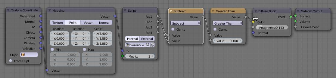
There still isn't but prompted by a question I decided to implement it in an ugly way; after all, if it works that is all that matters :-). All the necessary code to implement different distance metrics is already in node_texture.h but for some reason it was commented out. I therefore lifted the necessary part from this file and combined it with a a small shader that lets you choose the distance metric with an integer. An example for the Manhattan metric is shown below.

Node setup and code availability

The node setup used to generate the image above looks like this:

The code for the shader is available on GitHub. The node it generates may look a bit different than in the noodle shown here because I added an exponent input E that can be used for the generalized Minkovsky metric (metric == 6).

If you would like to know more about programming OSL you might be interested in my book "Open Shading Language for Blender". More on the availability of this book and a sample can be found on this page.

Greebles in OSL

The shader that is presented here basically takes as input a set of uv coordinates and produces a set of rectangles, each with their own uv coordinates. These rectangles are randomly distributed and rotated and do not necessarily cover everything: the fac output signals whether there is a rectangle or not.

With this set-up you can for instance cover a surface with random hull plates or similar:

The noodle used to produce the image looks like this:

There are two OSL shaders in this noodle: the first one on the left is called Greebles and is the one that divides up the coordinate space, the second one is called Rivets and is part of the green Rivets material layout. That last one simply distributes small circles around the edges of a rectangle.

Both shaders are available on GitHub, Greebles here, and Rivets here.

Strips OSL Shader: subdivide a uv map into strips and slots

In an ongoing effort to search for methods that can be used to generate bark textures I devised this simple OSL shader: it takes a uv-map (for example one that is wrapped around a cylinder representing a branch ans subdivides this in to strips. These strips are then subdivided into slots and each of these slots is given its own uv map and a random value.

This simple setup makes it possible for example to combine two tileable images in a manner that resembles bark an knots or cracks in that bark. The example below shows the result with two simple black and white images, mapped to a plane a a cylinder:

The underlying slots look like this:

Example node setup and code availability

The example node setup used to create both of the images above looks like this (click to enlarge):

The shader is availble on GitHub along with two sample textures: 1, 2.
The code should contain enough comments to get you going, but just tweaking the input parameters based on the example noodle should get you a long way.

Chaos mosaic with OSL

Chaos mosaic is a technique tht can be used to reduce the repetative appearance of tilebale images. An example is shown below. The upper right plane shows visible repetition artifacts that are not apparent in the lower left plane.

(I used a 700x700 tileable texture from CGtextures.com (Gravel0170_3_S.jpg) repeated four times in each direction on the upper right plane, and the same image with the chaosmosaic shader on the lower left plane)

Shader code

The shader code to implement this is very short:

shader chaosmosaic(
  point Pos=P,
  string Image="",
  int M=10,
  
  output color Color=0
){
  float x,y;

  x=mod(Pos[0],1);
  y=mod(Pos[1],1);
  
  float xi=floor(x*M);
  float yi=floor(y*M);
  
  // mapping here
  float xp=noise("cell",Pos,xi*M+yi);
  float yp=noise("cell",Pos,xi*M+yi+M*M);
  
  float xoffset = mod(mod(x,1.0/M)+xp,1);
  float yoffset = mod(mod(y,1.0/M)+yp,1);
  Color = texture(Image,xoffset,yoffset);
}

In the code above M is the number of squares in each direction in our uv map. We use it to calculate two indices (xi, and yi) that are subsequently used pick a random position in the texture (xp,yp). The pixel from the texture is then selected according to the relative offset in the small square inside the uv map (xoffset, yoffset). The original algorithm also uses a blending function between adjacent tiles form the textures but that will blur the image. In this case we didn't implement that because from far enough away the small tile edges aren't noticable but the large scale repetion has gone away so with very little code we already have a better result.

Example node setup

The node setup used for the example image (the plane on the lower left) looks like this:

reference

http://en.wikipedia.org/wiki/Texture_synthesis#Chaos_mosaic
http://research.microsoft.com/apps/pubs/?id=69770 (the research paper)

A hexagon shader in OSL, second edition

A while ago I made a simple OSL shader for hexagonal tilings. Prompted by some questions on BlenderArtists I decided to create a more versatile version that retained the color options but added the distance to the closest edge. That feature may help in creating crips edge patterns because the previously availble distance to the closest center creates rounded shapes that might be suitable for bee hives but not for hard edged stuff like floor tiles etc.

The noodle used to create the image is shown below (click to enlarge):

The color code has stayed the same except for the calculation of the distance to the edge. This might be a bit inefficient, but at least it's easy to read.
The additions are shown below, the full code is available on GitHub.

    // distance to nearest edge
    
    float x = mod(Coordinates[0]/3,1.0);
    float y = mod(Coordinates[1]/3,A2);
   
    #define N 18
    vector hc[N] = {
        vector(  0, -A2/3     ,0),
        vector(  0,     0     ,0),
        vector(  0,  A2/3     ,0),
        vector(  0,2*A2/3     ,0),
        vector(  0,  A2       ,0),
        vector(  0,4*A2/3     ,0),

        vector(0.5, -A2/3+A2/6,0),
        vector(0.5,     0+A2/6,0),
        vector(0.5,  A2/3+A2/6,0),
        vector(0.5,2*A2/3+A2/6,0),
        vector(0.5,  A2  +A2/6,0),
        vector(0.5,4*A2/3+A2/6,0),

        vector(1.0, -A2/3     ,0),
        vector(1.0,     0     ,0),
        vector(1.0,  A2/3     ,0),
        vector(1.0,2*A2/3     ,0),
        vector(1.0,  A2       ,0),
        vector(1.0,4*A2/3     ,0)
    };
    
    float d[N], t;
    
    for(int i=0; i < N; i++){
        float dx = x - hc[i][0];
        float dy = y - hc[i][1];
        d[i] = hypot(dx, dy); 
    }
    
    for(int j= N-1; j >= 0; j--){
        for(int i= 0; i < j; i++){
            if(d[i] > d[i+1]){ 
                SWAP(t, d[i], d[i+1]);
            }
        }
    }
    
    Center  = d[0];
    Edge    = d[1] - d[0];
    InEdge  = Edge < Width;

The approach we have taken is very simple: the hc enumerates all nearby hexagon centers. We then calculate all the distances to these points and sort them shortest to longest (yes with a bubble sort: with 18 elements it might just be faster to do it with a more efficient sorting algorithm at the cost of much more complex code so I don't bother).
The Edge is not realy the distance to the closest edge but the difference between the closest center and the next closest. Near the edge these values are more and more the same so Edge will approach zero. For convience we provide a comparison with some threshold also.

Settling of particles in suspension with Blender and OSL

Playing with volumetrics I wanted to approximate the effect of the settling of suspended particles from a fluid, like what happens when you leave a glass of orange juice standing for too long. The idea is that there is some region near the bottom of the glass that has a dense mass of settled particles and that in the beginning the diminishing density towards to surface is not all that visible but get clearer with time.
Of course this could be implemented with math nodes but I find it far simpler to write it all down in OSL and condense the logic in a single script node. The result shown below is admittedly not the animation that will get nominated for the next Academy Award but does show nicely the slow settling I had in mind, including the effect that near the end the fluid seems to clear up quicker:

OSL code and node setup

The node is simple enough:

shader edgedecay(
    point Pos    = P,
    float Edge   = 0.1,
    float Power  = 1,
    float Density= 10,
    float Length = 1 - Edge,
    
    output float Fac=Density
){
    float h = Pos[2];
  
    if(h>Edge){
        float d = (h - Edge)/Length;
        if(Power > 0 && d < 1){
            Fac = Density * ( 1 - pow(d,Power));
        }else{
            Fac = 0;
        }
    }
}

The node setup for the videoclip is:

The Density input was animated from 2.7 to 3.5 in 100 frames, while at the same time the Power input was animated from 1.0 to 0.0.
The following graph shows the plot of the density profile with relevant parameters:

A new tree addon, Part IV: volume rendering experiments with OSL

With the new volume shading options offered by Blenders OSL implementation it is tempting to try this on the trees generated by the space tree addon. Without adding any extra geometry or particles apart form a basic ahape a volume shader might give the impression of a much denser crown as shown in the image below:

This effect was achieved by inserting a scaled icosphere that covers about 90% of the crown interior (see below) and adding a volume shader to this icosphere that scatters and absorbs light in a non-uniform manner, i.e. the shader mimics a bunch of small scattered disks, which when seen from the distance add to the illusion of leaves. Note that we cannot do without all the leaves because volume scattering adds no specular reflections as real leaves might do.

Shader code and example node setup

The code for this shader consists of the shader proper, which merely checks which randomly scattered point we are closest to and then calls the indisk function with the position of this closest point and a random direction. indisk checks whether we are inside a disk with its axis in some direction and returns 1 if this is indeed so. Note that the include at the start of the code refers to a file that is distriubted with Blender and contains a number of useful functions, including a number of Voronoi/Worley related ones.

#include "node_texture.h"

int indisk(
  point p,
  point c, float r, float h, vector d
){
  vector v = p - c;
  float a = dot(v,d);
  float lh = abs(length(a * d));
  if(lh > h){ return 0;}
  float lv = length(v);
  float lp = sqrt(lv*lv - lh*lh);
  if(lp > r){ return 0;}
  return 1;
}

vector randomdirection(point p){
  float t = M_2PI*noise("cell",p,1);  
  float u = 2*noise("cell",p,2)-1;  
  float s,c,a;  
  sincos(t,s,c);  
  a = sqrt(1-u*u);  
  float x = a*c;  
  float y = a*s;  
  float z = u;  
  return vector(x,y,z);
}

shader bits(
  point Pos = P,
  float Scale = 1,
  float Size = 1,
  float Height = 0.05,

  output float Fac = 0
){
  point p = Pos * Scale;
  point centers[4];
  float distances[4];
  voronoi(p, "Distance Squared", 0, distances, centers);
  if(indisk(p,centers[0],Size,Height,randomdirection(p))){
    Fac = 1;
  }
}

The node setup to use this shader as seen in the opening image of this article looks like this:

Discussion

Whether using a volume shader this way is really useful remains to be seen: rendering this way is still rather slow. Of course, getting a comparable dense crown with extra particles also slows down rendering: in my tests doubling the number of particles from 1000 to 2000 resulted in a render time that was actually slower than adding the volume shader. In other words, your mileage may vary but it might be worth to experiment.

References

The space tree addon itself is introduced in a few articles on this blog and is available on GitHub. Relevant links are listed below:

wiggles / noodles shader for OSL

The basic idea of this shader is to scatter around wiggly lines that can be used as fibers, hairs or, like in the image below, noodles.

Each line consists of a number of segments connected end to end. Each segment is angled by a random amount relative to the previous one. Segments are not straight though, but curved by a certain amount. The parameters that control the shape of the line are illustrated below, with on the right an indication of what the basic pattern looks like:

The curved segments are implemented as quadratic splines, using routines discussed in an earlier article.

Code and node setup

The code is pretty straightforward. Apart from a rather long list of input parameters it is mainly concerned with calculating a list of segments for each line we want to draw (there may be more than one per cell). The main trick is in line 86, where we make certain that point p1, the point that is used to control the curvature of each segment, lies on the line line through the previous control point and the end point. This ensures that each segment joins the previous one smoothly.

#include "equations.h"

#define DOT(a,b) (a[0]*b[0]+a[1]*b[1])
#define SUB(a,b) vector(a[0]-b[0],a[1]-b[1],0)

// determine if point M is inside a rectangle with a margin
int in_rectangle(point M, point a, point b,
  vector u, float W, vector v, float linewidth){
  point A=a+linewidth*(-u-v);
  point B=b+linewidth*(u-v);
  point D=B+(W+2*linewidth)*v;
  vector AM=SUB(M,A);
  vector AD=SUB(D,A);
  vector AB=SUB(B,A);
  float dotamad=DOT(AM, AD);
  float dotadad=DOT(AD, AD);
  float dotamab=DOT(AM, AB);
  float dotabab=DOT(AB, AB);
  return (dotamad > 0 && dotamad < dotadad) && 
         (dotamab > 0 && dotamab < dotabab);
}

#define CELL noise("cell", cp, seed++)
#define CELL2 vector(CELL, CELL, 0)

shader wiggles(
  point Pos=P,
  float Scale=1,

  int Number=1,

  float Length=0.5,
  float LengthVar=0,
  float Kink=0,
  float Curl=0.2,
  float Wave=30,    // degrees
  int Steps=2,
  float StepsVar=0,

  float Width=0.02,
  float WidthVar=0,

  int Seed=0,
  
  output float Fac=0
){
  point p = Pos * Scale;
  p[2]=0;
  point ip= point(floor(p[0]),floor(p[1]),0);

  int nn=1+(int)ceil(Steps*Length);

  for(int xx=-nn; xx <= nn; xx++){
    for(int yy=-nn; yy <= nn; yy++){
      int seed=Seed;
      point cp = ip + vector(xx, yy, 0);
      for(int wiggle=0; wiggle < Number; wiggle++){
        vector start = cp + CELL2;
        start[2]=0;
        vector dir = CELL2 - 0.5;
        dir[2]=0;
        dir = normalize(dir);
          
        vector perp = vector(dir[1],-dir[0],0);
        float k=0.5 + Kink * (CELL-0.5);
        float c=Curl*(CELL-0.5);
        point p1=start+k*dir+c*perp;
        for(int step=0; step < Steps; step++){
          vector ldir = dir;
          ldir *= Length + LengthVar*CELL;
          point end=start+ldir;
          if(in_rectangle(p, start, end, dir, c/2, perp, Width+WidthVar)){
            float d,t;
            if(splinedist(start, p1, end, p, d, t)){
              float localwidth = Width+WidthVar*noise("uperlin",start,t);
              if(d < localwidth){
                Fac = (localwidth - d)/localwidth;
                return;
              }
            }
          }

          if(CELL < StepsVar){
            break;
          }else{
            p1 = end + (end - p1)*(1+noise("perlin",end)*Kink); 
            start = end;
            dir = rotate(dir, radians(Wave*noise("perlin", start)), vector(0,0,0), vector(0,0,1));
          }
        }
      }
    }
  }
}

The only other issue that needs attention is the generation of random numbers. In each cell we need a number of them and they need to be unique. We therefore add an extra seed argument to the call to noise. However, we must take care that all those numbers are generated in a repeatable way so we reset this seed for each cell to the value provided by the Seed input. This allows us to generate unique patterns for different objects sharing the same material.
The example image at the start was created with a node setup like this:

Note that the Fac output isn't simply 1 or 0 but contains the distance to the edge of the fiber and we use that to drive a bump node (through a square root math node (power 0.5) to give it a smoothly curved appearance). We use the object info node to generate a random number because the heap of noodles consists of three separate squashed half spheres. The shader expects an integer so we multiply the random value by a million to get a unique integer.
One final node of caution: this isn't a cheap shader because calculating the distance to a spline is rather expensive. OSL is quite good at optimizing expressions but still I did dpend quite some time on optimizing the splinedist() by hand. Did did indeed shave off some small percentage but the biggest win was the conversion of all calculations to two dimensions and the test to see if we are within the bound of the control rectangle before actually checking the distance to the spline (line 72 in the code)
A final thing is that most random vectors we generate don't need the z component but OSL has no notion of 2D vectors. I rewrote that in a way that doesn't waste a third of the random values calculated (the CELL2 macro). Even with these optimizations the image with the noodles took an hour to render (200 samples on a hexacore machine). That might be a bit too much but for adding realism to a sweater (in my case that means with cat hairs all over it ;-) this might be a interesting opton.

Code availability

The code is available on GitHub. For ease of use I inlined the necessary functions from equations.h so the shader can be used as is, without external dependencies.

An OSL wood shader with knots for Blender Cycles

In a previous article I presented a shader that could be used to create the impression of knots in wood. This was accomplished by warping the texture coordinates around randomly distributed points in space.

Knots however do not resemble spheres but are more like cylinders that are cut under a slight angle. This distinction is not that important but for completeness sake we present this new implementation here together with a node setup that combines these knots with the wood shader we presented a while ago. An example result is shown below.

Code and example node setup

The implementation differs from the previous one in generating random lines (represented by a random point plus a random direction) instead of points. The texture coordinates are bent proportional to the distance to the closest point on this random line, so the bend() is a little bit more complicated than before.


vector random_sphere(point p, int n, float zdistribution){  
  float t = M_2PI*noise("cell",p,n*2+0);  
  float u = 2*noise("cell",p,n*2+1)-1;  
  float s,c,a;  
  sincos(t,s,c);  
  a = sqrt(1-u*u);  
  float x = a*c;  
  float y = a*s;  
  float z = u*zdistribution;  
  return vector(x,y,z);    
}

int bend(vector p, vector k, vector kv, float r, float a, float m, output vector B){
  vector pk = k - p;
  vector t = dot(pk,kv)/dot(kv,kv);
  vector D = k + t * kv - p;
  float L = length(D);
  if( L < r ){
    float c = L/r;
 float d = m * pow( 1 - c , a);
 if( d < L ){
  B = d * normalize(D);
  return 1;
 }else{
     B = D;
  return 2;
 }
  }
  return 0;
}

shader knot(
  vector Pos = P,
  float Scale = 1.5,

  float R = 2.9,
  float Falloff = 2,
  float Strength = 1,
  float Knots=0.1,
  float Z=1,
  
  output vector Vec = P,
  output float Fac = 0
){
  vector p = Scale * Pos;
  vector sdp = 0;

  float TR = ceil(R);
  for(float dx=-TR; dx <= TR; dx++){
    for(float dy=-TR; dy <= TR; dy++){
      for(float dz=-TR; dz <= TR; dz++){
        vector ip = floor(p)+vector(dx,dy,dz);
        for(int ik=0; ik < (int)Knots; ik++){
          vector k = noise("cell",ip,ik);
    vector kv= random_sphere(ip,ik+1000,Z);
          vector dp= 0;
    int ret = bend(p,ip+k,kv,R,Falloff,Strength,dp);
          if(ret != 0){
            Fac=max(Fac,ret==2);
            sdp+=dp;
          }
        }
        if( noise("cell",ip,-1) < mod(Knots,1.0) ){
          vector k = noise("cell",ip,-2);
    vector kv= random_sphere(ip,998,Z);
          vector dp= 0;
    int ret = bend(p,ip+k,kv,R,Falloff,Strength,dp);
          if(ret != 0){
            Fac=max(Fac,ret==2);
            sdp+=dp;
          }
        }
      }
    }
  }
  if( Fac < 1 ){
 Vec = p + sdp;
  }else{
    Vec = sdp;
  }
}

Note that the function random_sphere() is modified from the one presented in a previous article to bias the vectors that are returned. This allows us to tweak the orientation of the generated knots, which might give more realisted results because branches (the source of the knots) are not pointing in all directions from the stem.

The node setup used to create the material in the example image is shown below (click to enlarge).

Room for improvement

The distribution of the knots might be convincing enough for our purposes but the material is now just another (darker) wood mzterial, rings and all. Quits a number of wood knots do look like that but a significant fraction shows characteristic radial cracks. This is caused when the wood is dried because the material properties of the knot are different from the surrounding wood. It would be nice if we could implement this in some way as well.

OSL leaf veins shader for Cycles

When we look at images the addition of veins greatly adds to the preceived realism of rendered leaves and in this article I present a simple veins shader that complements the leaf shader discussed previously.

Leaf veins

I forgot to update the page that describes equations.h (thanks samblerdevel for pointing that out). I just corrected that so if you had any errors complaining abot a function splinedist() that was missing, download & install equations.h and try again

The node setup used to create the leaf shape and veination in the close-up image above is relatievely complicated and presented at the end of this article. Luckily, the basic stuff of generating vein patterns is not that complicated so lets have a look at that first.

As illustrated in the images above the veins in the leaf are all represented by cubic splines, starting at the red dots on the central vein and curving to the green end points on the edge of the leaf. Their curvature is controled by the blue control points. A node setup for the image above looks like this:

The Angle and L parameters mimic the ones in the leaf shape shader and are kept the same in this case to let the endpoints of the veins coincide with the actual leaf edge. The number of veins, their distribution, width and the way they curve are controlled by the Veins, Width, Squish and Up parameters as we will see later on. Their is some randomness in the placement as well which can bee influenced by the Seed and Var parameters. The outputs consist chiefly of a Vein socket which will be one for a vein, and a Fac socket which is the square root of the distance to the center of the vein and can be used to drive displacement.

The code for this node is shown below makes use of the equations.h include discussed in the article on leaf shapes.


#include "equations.h"

shader arcuateveins(
 point Pos = P,
 int Veins = 7,
 int Seed = 42,
 float Var = 0,
 float Width = 0.05,
 float NWidth = 0.25, // size of the reticulated area
 
 float Squish  = 0.5, // distribution of endpoints on edge
 float Squish2 = 0.5, // distribution of controlpoints
 float Squish3 = 0.5, // distribution of starting points
 float Up = 0.5,
 
 float Angle1 = 70,
 float L1 = 1,
 float Angle2 = 70,
 float L2 = 1,
 
 output float Vein = 0,
 output float Net = 0,
 output float Fac = 0
){

 float delta = 1.0/((float)Veins+1);
 float delta2= delta/2;
 float delta4= delta/4;
 
 // calculate the four control points of the cubic spline that defines the leaf edge
 float x1,y1,x2,y2;
 sincos(radians(Angle1),y1,x1);
 sincos(radians(Angle2),y2,x2);
 point P0 = point(0      , 0 ,0);
 point P1 = point(x1     , y1,0)*L1;
 point P2 = point(1-x2*L2, y2*L2,0);
 point P3 = point(1      , 0 ,0);
 
 point P0q = point(P0[0],P0[1]*Up,P0[2]);
 point P1q = point(P1[0],P1[1]*Up,P1[2]);
 point P2q = point(P2[0],P2[1]*Up,P2[2]);
 point P3q = point(P3[0],P3[1]*Up,P3[2]);
 
 int i;
 for(i=0;i < Veins;i++){

  // determine the starting points of the veins
  float x = (i*delta+delta2*Var*cellnoise(i+10+Seed))*Squish3;
  float dx = (delta4*Var*cellnoise(i+17+Seed))*Squish3;
  point P0up   = point(delta2+x+dx,0,0);
  point P0down = point(delta2+x,0,0);
  // determine the endpoints on the leaf edge
  float t=(i*delta+delta2)*Squish+1-Squish;
  point P2up   = cubicspline(t,P0,P1,P2,P3);
  point P2down = point(P2up[0],-P2up[1],P2up[2]);
  // the veins are quadratic splines, so need one additional control point
  t=(i*delta+delta2)*Squish2+1-Squish2;
  point P1up   = cubicspline(t,P0q,P1q,P2q,P3q);
  point P1down = point(P1up[0],-P1up[1],P1up[2]);
  
  float r;
  int f = splinedist(P0up, P1up, P2up, Pos, r, t);
  if ( f && (r < NWidth ) ) Net = 1 ;
  if ( f && (r < Width * ( 1- t) * (1-Pos[0]) ) ) { Vein = 1; Fac = sqrt(1-r/Width); break; }
  f = splinedist(P0down, P1down, P2down, Pos, r , t);
  if ( f && (r < NWidth ) ) Net = 1 ;
  if ( f && (r < Width * ( 1- t) * (1-Pos[0]) ) ) { Vein = 1; Fac = sqrt(1-r/Width); break; }
 }
 
 // the central vein
 float d = distance(point(0,0,0),point(1,0,0),Pos);
 if ( d < NWidth ) Net = 1 ;
 if (d < (Width * (1-Pos[0])) ) { Vein = 1; Fac = sqrt(1-d/Width);}
}

Relation to real venation patterns in leaves

The shader in its current form is able to model pinnate and arcuate venation patters and intermediate forms of these. (For an explanation of terminolgy refer to Wikipedia, especially this overview sheet). Its spline-based modelling of the veins is not based on any underlying theory of the formation of veins as it happens in nature, as these reaction-diffusion equations cannot so easily be implemented in an OSL shader (at least not at present: we wouldn't want to redo such a costly simulation again and again for each point being shaded so we would need peform the simulation before we start shading each pixel. Currently there is no facility for adding something to a shader that will be executed once beforehand, although there might be in the future. An alternative approach might be to perform the simulation, maybe in a Python add-on, and store the result in a texture. Here we opted for art before science: if it looks all right we don't care what it is based on).

Controlling the curve shape of the veins

In the following images I have illustrated how you can control the shape of the veins. How much the starting points on the central vein and the control points in the middle and the end points on the leaf edge are bunched up, is controlled by the Squish parameters. The blue control points all lie on a spline that is a copy of the spline that defines the leaf edge by scaled by the Up parameter. Some experimenting shows that is is possible to create both pinnate venation patterns as well as arcuate patterns:

Example node setup

The leaves in the image at the top of this article were created with the following node setup:

The values in the blue box simultaneously control the shape of the leaf edge both in the leaf shader and in the vein shader. The leaf coloring is controled by the nodes in the green box (leaves are both glossy and translucent) while the vein coloring is is defined by the nodes in the red box, the choice being determined by the Vein output socket of the vein shader. The yellow box provides some noisy patterns to drive both the colloration of the leaf as well as mix with the bump patern from the vein shader to drive the displacement. The exact contribution of these displacements is controlled by the purple nodes.

Room for improvement

Although the shader is already quite versatile there is ample room for imrpovement. For example, I would like it to be able to produce palmate vein patters and to control the narrowing towards the tips of the veins. On the other hand the shader is not limited to producing vein pattersn: I imagine it can be used to produce fish bones and bird feather patterns (barbs) as well. I might expand on that in the future.

An OSL Wood Shader for Blender Cycles

Good looking procedural wood is not that simple to implement but fortunately for us their is a whole host of renderman shading experience available online. Based on a shader by Larry Gritz we implement a fairly realistic wood shader in OSL.

Both the dark wood of Suzanne and the torus and the lighter wood of the planks they are resting on was done with the shader we present in this blog article. The algorithms used to produce the ring and the grain are essentialy the same as those implemented in Larry Gritz' oak shader. However, Open Shading Language (OSL) is not quite the same as Renderman so there was in the end quite some adaptation needed.

Beside syntactic differences between RSL and OSL, the main differences are that OSL provides us natively with snoise() functions but on the other hand, a function like area() doesn't seem to work well and neither are the derivative functions. However, because of the inherent antialiasing in Cycles we don't have to bother much about filter width (as we would have in other types of render engines) so we can do without I think. Functionally the biggest adaptation was that the original implementation provided a complete lighting model (a closure) for the wood shader while we adopt a more modular approach provinding color and displacement output that can be combined with existing closures for maximum flexibility. See the node setup at the end of the article for an example.

The code is for the OSL shader is shown below. Implementation mistakes are mine but the credits go to Larry Gritz:


// for the original renderman shader, check http://www.larrygritz.com/arman/materials.html

// adapted from larry gritz advanced renderman patterns.h
float smoothpulse (float e0, float e1, float e2, float e3, float x)
{
    return smoothstep(e0,e1,x) - smoothstep(e2,e3,x);
}

/* A pulse train of smoothsteps: a signal that repeats with a given
 * period, and is 0 when 0 <= mod(x/period,1) < edge, and 1 when
 * mod(x/period,1) > edge.  
 */
float smoothpulsetrain (float e0, float e1, float e2, float e3, float period, float x)
{
    return smoothpulse (e0, e1, e2, e3, mod(x,period));
}

// adapted from larry gritz advanced renderman noises.h
/* fractional Brownian motion
 * Inputs: 
 *    p     position
 *    octaves        max # of octaves to calculate
 *    lacunarity     frequency spacing between successive octaves
 *    gain           scaling factor between successive octaves
 */

/* A vector-valued antialiased fBm. */
vector vfBm (point p, float octaves, float lacunarity, float gain)
{
    float amp = 1;
    point pp = p;
    vector sum = 0;
    float i;

    for (i = 0;  i < octaves;  i += 1) {
  vector d = snoise(pp);
  sum += amp * d;
  amp *= gain;  
  pp *= lacunarity;  
    }
    return sum;
}

// adapted from larry gritz oak.sl and oak.h
// original comments between /* ... */
// my comments start with //
// note that I dropped the whole filterwidth stuff, partly 
// because I don't think it necessary in Blender Cycles, partly
// because the derivatives and area() function doesn't seem to work (yet)
// all specialized snoise defines are replaced by snoise() function calls
float oaktexture (point Pshad,
  float dPshad,
  float ringfreq, 
  float ringunevenness, 
  float grainfreq,
     float ringnoise, 
  float ringnoisefreq,
     float trunkwobble, 
  float trunkwobblefreq,
     float angularwobble,
  float angularwobblefreq,
     float ringy, 
  float grainy)
{
    /* We shade based on Pshad, but we add several layers of warping: */
    /* Some general warping of the domain */
    vector offset = vfBm(Pshad*ringnoisefreq, 2, 4, 0.5);
    
 point Pring = Pshad + ringnoise*offset;
    /* The trunk isn't totally steady xy as you go up in z */
 vector d = snoise(Pshad[2]*trunkwobblefreq) ;
    Pring += trunkwobble * d * vector(1,1,0);

    /* Calculate the radius from the center. */
    float r = hypot(Pring[0], Pring[1]) * ringfreq;
    /* Add some noise around the trunk */
    r += angularwobble * smoothstep(0,5,r)
    * snoise (angularwobblefreq*(Pring)*vector(1,1,0.1));

    /* Now add some noise so all rings are not equal width */
    r += ringunevenness*snoise(r);

    float inring = smoothpulsetrain (.1, .55, .7, .95, 1, r);

    point Pgrain = Pshad*grainfreq*vector(1,1,.05);
    float dPgrain = dPshad; //dropped filterwidthp(Pgrain);
    float grain = 0;
    float i, amp=1;
    for (i = 0;  i < 2;  i += 1) {
 float grain1valid = 1-smoothstep(.2,.6,dPgrain);
 if (grain1valid > 0) {
     float g = grain1valid * snoise (Pgrain);
     g *= (0.3 + 0.7*inring);
     g = pow(clamp(0.8 - (g),0,1),2);
     g = grainy * smoothstep (0.5, 1, g);
     if (i == 0)
  inring *= (1-0.4*grain1valid);
     grain = max (grain, g);
 }
 Pgrain *= 2;
 dPgrain *= 2;
 amp *= 0.5;
    }

    return mix (inring*ringy, 1, grain);
}

// larry gritz' original shader was a closure but this shader
// provides different outputs that you can plug into your own
// closures/shaders
surface oak( 
   point Pos = P,
   float Sharpness = 0.01, // sharpness of the grain. hand tweaked because we lack derivatives.
   float ringfreq = 8, 
   float ringunevenness = 0.5,
      float ringnoise = 0.02, 
   float ringnoisefreq = 1,
      float grainfreq = 25,
      float trunkwobble = 0.15, 
   float trunkwobblefreq = 0.025,
      float angularwobble = 1, 
   float angularwobblefreq = 1.5,
      color Clightwood = color(.5, .2, .067),
      color Cdarkwood = color(0.15, 0.077, 0.028),
      float ringy = 1, 
   float grainy = 1,
      output color Color = 0,
   output float Spec = 0.1,
   output float Roughness = 0.1,
   output float Disp = 0
    )
{
    float wood = oaktexture (Pos, Sharpness, ringfreq, ringunevenness, grainfreq, 
         ringnoise, ringnoisefreq, trunkwobble, trunkwobblefreq,
         angularwobble, angularwobblefreq, ringy, grainy);
    
 Color = mix (Clightwood, Cdarkwood, wood);
    Disp = -wood;  // lightwood = 0, darkwood is deeper/lower = -1
 Spec = 0.1*(1-0.5*wood); // darkwood is less specular
 Roughness = 0.1+0.1*wood; // and rougher
}

Example node setup

The node setup for the Suzanne and the torus looks like this:

A chainmail OSL shader in Blender Cycles

A golden oldie reimplemented in OSL: a simple 4-in-1 chainmail pattern.
If you want to know more about chainmail patterns, both historical and contemporary ones, you might like to visit artofchainmail.com or cgmaille.com.

In the picture ob the left I used the chainmail shader to generate the pattern on the neck flap. The picture was created with a wood texture from cgtextures.com for the table top but all other textures are procedural. The scene was lit using the Prov-Wash HDRI maps by Alex Hart as found on hdrlabs.com. I think it is a kind of museum and that fits the helmet setting nicely.
Like the barbwire and chainlink shaders the shader presented in this article is again essentially nothing more than a simple black and white pattern with the distance to the center of the line added as a feature to aid in generating bumps. The difficulty here is to get all those overlaps correct as can be seen in the enlarged cut out selection shown on the right.

#include "stdosl.h"

int between(float v, float a, float b){ return v >= a && v <= b; }
float arc(float r, float a, float b) { return sqrt(0.5-abs(0.5-((r-a)/(b-a)))); }
float rmap(float a, float b, float ra[3] ){
 if ( between(ra[0], a, b) ) { return ra[0]; }
 if ( between(ra[1], a, b) ) { return ra[1]; }
 if ( between(ra[2], a, b) ) { return ra[2]; }
 return -1;
}

float basepattern(float r1, float r2, float r3, int fx, int fy, float Rm, float Rp){
 float x0y0[3] = {r3, r1, r2};
 float x0y1[3] = {r2, r3, r1};
 float x1y0[3] = {r1, r3, r2};
 float x1y1[3] = {r2, r1, r3};
 
 float r = -1;
 if ( fx ){
  if ( fy ) {
   r = rmap(Rm, Rp, x1y1);
  } else {
   r = rmap(Rm, Rp, x1y0);
  }

 } else {
  if ( fy ) {
   r = rmap(Rm, Rp, x0y1);
  } else {
   r = rmap(Rm, Rp, x0y0); 
  }
 }
 return r;
}

shader chainmail4in1 (
 point Pos = P,
 float Scale = 1,
 float Radius = 0.47,
 float Width = 0.08,
 output float Fac = 0,
 output float Disp = 0
){
 point p = Pos * Scale ;
 float x = mod(p[0],1);
 float y = mod(p[1],1);
 
 float Rm = Radius - Width;
 float Rp = Radius + Width;
 
 float r=-1,r1,r2,r3,cr1,cr2,cr3;
 
 int fx = 0, fy = 0 , flip = y > x, flipt = y > ( 1 - x );
 if ( x > 0.5 ){ x = 1 - x ; fx = 1; }
 if ( y > 0.5 ){ y = 1 - y ; fy = 1; }
 
 r1 = hypot(x-0.5,y-0.5);
 r2 = hypot(x-0.5,y+0.5);
 r3 = hypot(x+0.5,y-0.5);
 
 float xc = mod(p[0]+0.5,1);
 float yc = mod(p[1]+0.5,1);
 
 int fxc = 0, fyc = 0, flipc = y > x;
 
 if ( xc > 0.5 ){ xc = 1 - xc ; fxc = 1; }
 if ( yc > 0.5 ){ yc = 1 - yc ; fyc = 1; }
 
 cr1 = hypot(xc-0.5,yc-0.5);
 cr2 = hypot(xc-0.5,yc+0.5);
 cr3 = hypot(xc+0.5,yc-0.5);

 if ( flip ^ flipt ){
  // base pattern
  r = basepattern(r1,r2,r3,fx,fy,Rm,Rp);
  if ( r> -1){
   Fac = 1;
   Disp = arc(r,Rm,Rp);
  } else {
   // connecting rings
   r = basepattern(cr1,cr2,cr3,fxc,fyc,Rm,Rp);
   if ( r> -1){
    Fac = 1;
    Disp = arc(r,Rm,Rp);
   }
  }
 } else {
  // connecting rings
  r = basepattern(cr1,cr2,cr3,fxc,fyc,Rm,Rp);
  if ( r> -1){
   Fac = 1;
   Disp = arc(r,Rm,Rp);
  } else {
   // base patterm
   r = basepattern(r1,r2,r3,fx,fy,Rm,Rp);
   if ( r> -1){
    Fac = 1;
    Disp = arc(r,Rm,Rp);
   }
  }
 }
}

The trick is to see that the pattern is very symmetrical. Each quadrant is basically the aame and consists of two quarter ring segments, one centered on the center of the square we are filling, the other one on the corner. The whole business of which to test for in what order is done to make sure that we know which ring segment is on top so that we can calculate a displacement correctly. It is all a bit too complicated to explain and in fact the code was created on a trial and error basis :-) It is however quite simple to use and that's why I share it of course :-)

Example node setup

Like most of the shaders I present on this blog the pattern probably is easiest to work with on an uv-mapped object. In the picture of the helmet the neckflap is just that, a curved, subdivided square that is uv-mapped with simple unwrapping. The node setup is shown below.

The green part is where we switch between a fully transparent shader or a metal shader based on the ouput of our script node. The diffuse part of the metal shader is given some color variation by the noise generated in the red box. The blue box s where we perturb our uv-coordinates a little bit adding a small amount of color noise in order to make our chainmail pattern a little less regular.

How to set up simple hdri environment lighting in Blender Cycles

In quite a few articles on this blog I present example images that use environment lighting and a detailed backplate. I found it not very intuitive at first to set up a scene in a way that gave me some control so I thought I'd share my findings here.

When using environment lighting with backplates you need of course have access to good resources and one of the best free resources I found is the sIBL Archive on hdrlabs.com. Each archive contains normally three images: a high resolution backplate, a low resolution hdri environment map and a high resolution hdri reflection map, all in a format that can be used by Blender directly. Just make sure you use an Environment Texture node (not a regular imaged texture). The environments we use here are all equilateral but Blender also has the option to use mirror ball images.

A high resolution (8000 x 4000 pixels) backplate is already huge and an hdri image is even bigger (typically 4 to 10 times) both because it uses more bits to store the information in each color channel and because it appears to compress less well. It would be wasteful to keep all this in memory if you don't need it because memory already is a precious commodity when rendering. Therefore each map has a different resolution: the backplate is very detailed, but is plain rgb, not hdri, and the environment map is very low resolution since you won't see it directly and lights don't need fine detail. In reflections however you might need some detail (if you have very shiny surfaces where you can see the environment) and in that case you might want to use the medium resolution reflection maps. In the image at the start of the article I used the low resolution enviroment map and as you can see the very glossy monkey on the right doesn't show a recognizable image in the reflection. In the image below we used a medium resolution reflection map which gives fair result while still being much smaller than an hdri map with the same resoltion as the back plate would be.

If we can see the background we have to create a setup for the world material nodes where we couple the highly detailed background image to the lower resolution environment or reflection map, in such a way that when we look a the background directly we see the backplate while in all other cases (like diffuse and specular reflection bounces for example) we use the hdri map. This is possible by using Cycles' light path node.

The light path node has an Is Camera Ray socket that will have a value of one if we are dealing with a camera ray and is zero otherwise. A camera ray is a ray that shoots directly from the camera so if our background is hit by a camera ray we present the high res backplate and in all other cases we present the hdri environment map. This is done by drivin the mix shader in the node setup above by this camera ray. Note that the backplate shader is the one that plugs into the lower input socket of the mix shader.

When you create your scene it is convenient to place your camera in the center, i.e. at location 0,0,0 because these environment images are shot like a panorama with the real world camera in its center. This doesn't have to be exact but in indoor scenes some distortion might be noticeable if you rotate the camera while it is not in the center.

Now if you want to change your view and lighting you could rotate the camera but then you would need to move all other objects as well. It might be much more convenient to rotate the background imagery. The backplate and the environment map will have to be linked of course to keep what you see and how things are lit in sync and the easiest way to do that is shown in the node setup below

The generated coordinates are fed through a vector mapping node before being connected to both background shaders. We now can rotate both images at the same time by changing the z-rotation value of the mapping node. (The other roatations are generally less useful as in these good quality pictures there is hardly ever the need to correct a tilted horizon for example but if need this could be done by rotating around the x or y axis).

A fingerprint OSL shader for Blender Cycles

Scanning your own fingerprints for use in your renderings might not be such a good idea with new methods of identity theft being invented everyday so here I present a shader that generates random fingerprint patterns. Finally you can identify the suspect that emptied your whiskey glass!

In the example image we duplicated and separated a small square from the glass mesh and scaled it a minuscule bit outward, effectively turning it into a decal or sticker. This object was uv-mapped and the fingerprint material applied to it. (The decal is still a bit darker than the glass because I didn't use enough transparent bounces. I might update this image in the future.)

An elliptic mask shader

Besides the regular nodes this Cycles shader consist of two separate OSL shaders. The first is a generic one to generate elliptic masks, not unlike the one available in the compositor:

#include "stdosl.h"

shader ellipse(
 point Pos = P,
 point Center = 0.5,
 float Radius = 0.5,
 float E = 1,
 float Rotation = 0,
 float Blur = 0,
 output float Fac = 0
){
 point p = rotate(Pos,radians(Rotation),Center,Center+vector(0,0,1));
 vector d = p - Center;
 d[0] *= E;
 float r2 = d[0]*d[0]+d[1]*d[1];
 if (r2 <= Radius*Radius) {
  Fac = 1-Blur*sqrt(r2/(Radius*Radius));
 }
}

Generating a flow field

The second one is a flow shader. It works by generating a number of points that are considered the centers of vortices (rotating vector fields) with different strengths. At the point being shaded all the vectors are summed and the magnitude of the resulting vector is calculated. This output is used in the example noodle at the end of this article as input to a sinus node to create the banding pattern. Of course this pattern only superficially resembles human fingerprints (for example, it will not produce whorls, just concentric circles) but it does resemble it and is in fact related to the way fingerprint patterns are produced in the developing embryo. Anyway, as always, shaders are not about science but about art. For more information check Wikipedia, this pdf or this research. The animation on that last site actually inspired me although I have no idea my simplistic implementation in any way resembles their approach apart from using a vector field to act as a base for generating the ridge patterns.
Apart from fingerprints I think it should be possible to generate all sorts of patterns that in real life might be produced by processes that resemble cellular automata or reaction-diffusion systems that are far too expensive to simulate insode a shader. Zebra stripes might be a prime example.
I think my approach is at generating these patterns for graphical purposes is quite new, but if you have pointers to similar solutions you saw elsewhere, please mention this is a comment.

#include "stdosl.h"
#include "node_texture.h"

shader flow(
 point Pos = P,
 float Scale = 1,
 int Np = 5,
 int Seed = 42,
 output float Fac = 0
){
 float da;
 point pa;
 float d;
 
 vector up   = vector(0,0,1);
 vector tdir = 0;
 
 int pi;
 
 for(pi=0; pi< Np; pi++){
  pa = Scale * point(
   cellnoise(point(pi,pi,pi)),
   cellnoise(point(pi,pi+Seed,pi)),
   cellnoise(point(pi,pi,pi+Seed)));
  da = pa[2];
  vector v = pa - Pos;
  float d = length(v);
  v[2]=0;
  v = normalize(v);
  tdir += cross(v,up)*da*d;
 }
 Fac = sqrt(dot(tdir,tdir));
}

If we use some lighting that shows of the details you can see that it resembles a fingerprint but is actually nowhere near a real one.

Example node setup

The are quite a few nodes in the example shown below, so it is good the understand the general flow. The flow shader is used drive a sinus node via a multiplication node that lets us control the spacing of the bands. The output of this sinus is only propagated if it is positive (that is what the greater than and multiply nodes do, akin to an electrical 'rectifier' circuit) [The red box]]. This is mutiplied (i.e. masked) by the output of the ellipse shader and again by some noise [both in the green box] before being fed into mixture of closures (shaders) that will turn complete transparent when black and whitish-with-a-slight-gloss if not black [the yellow highlight]. The sinusoidal ridges also drive the displacement, adding a little extra realism [the blue highlight].

A Barbwire OSL shader for Blender Cycles

The simple concept used to create a chain link fence is easily extended to a somewhat more elaborate shader that creates barbwire. Finally we can keep the farm animals out of our rendered gardens (but as a goat owner myself I do not really think you should use barbwire to keep animals out except for humans :-)

I won't claim that the composite is very good, but the barbwire material itself holds up quite well even fairly close up.
In the example image I used the sIBL HDRI set 'Topanga Forest B' from Blochi as found on the sIBL archive and for the wooden posts some textures from CGTextures.
The code for the shader is pretty tangled, mainly because the spikey bit of the barbwire is pretty hard to code. The Xscale input is provided in order to make it possible to reduce the number of spikes per length of wire. By default we generate one spike per two turns. If you want to reduce this, you increase the number of turns, scale your input position in the x-direction and divide the Xscale input by the same amount (otherwise the turns on the spike would scale along and look way to thick).

#include "stdosl.h"

float arc(float r){ return sqrt(0.25-(r-0.5)*(r-0.5)); }

shader barbwire(
 float Width = 0.05,
 int Turns = 2,
 int Spiketurns = 2,
 float Xscale = 1,
 point Pos = P,
 output float Fac = 0,
 output float Displ = 0
){
 float x = mod(Pos[0],1);
 float y = mod(Pos[1],1);
 
 if ( x > 0.5 ) {
  x = 1 - x;
  y = 1 - y;
 }
 
 float w = Width/2;
 float t = M_2PI*x*Turns;
 
 float c = cos(t);
 float h = c*w+w;
 float l = c*w-w;
 
 y -= 0.5;
 // the barb part
 float BWidth = Width*Xscale;
 float Lw = BWidth*(Spiketurns-1);
 float Hw = BWidth*Spiketurns;
 if ( x > Lw && x < Hw && y > 1.5*Width && y<4 br="" idth="" part="" spikey="" the="">  if( y<3 br="" idth="" x-width="" y-3="">   Fac = 1;
   Displ = arc(mod(x,BWidth)/BWidth);
  }
 } else if ( x < Hw && abs(y) < 2*Width ){
  if ( abs(y) > 1.5*Width) { // the rounded top and bottom parts
   if ( abs(y) - 1.5*Width < w*arc(mod(x,BWidth)/BWidth) ){
    Fac = 1;
    Displ = arc(mod(x,BWidth)/BWidth);
   }
  } else { // the main part
   Fac = 1;
   Displ = arc(mod(x,BWidth)/BWidth);
  }
 }
 // the wire part 
 else {
  // alternating top/bottom checks to get correct crossings
  if ( (int)(t/M_PI) % 2 == 1 ){
  
   if ( y > l && y < h ) {
    Fac = 1;
    Displ = arc((y-l)/Width);
   } else if ( -y > l && -y < h ) {
    Fac = 1;
    Displ = arc((-y-l)/Width);
   }
   
  } else {
  
   if ( -y > l && -y < h ) {
    Fac = 1;
    Displ = arc((-y-l)/Width);
   } else if ( y > l && y < h ) {
    Fac = 1;
    Displ = arc((y-l)/Width);
   }
  }
 }
}

Example node setup

In the example image at the start of this article the lengths of barbwire were modelled by creating a single square, uv-unwrapping it and then adding an array modifier and a curve modifier to this square. This way we could edit the curve anyway we liked while the square repeats itself as many times as necessary (I set the length of the array modifier to the the length of the same curve that was used in the curve modifier). The noodle that applies the barbwire segment to the square looks like this (it is basically the same as the one for the chain link fence shader):

A 4D voronoi OSL shader for Blender Cycles

I took a post on Blender Artists as a challenge and created a 4D voronoi shader.

Blogspot won't show animated gifs but I put up a short sequence on PasteAll and if that doesn't work it is also on my site. In this animated gif, the fourth dimension (time) is animated from 0 to 1 in 50 frames.
The shader presented below is simple enough but convoluted because we cannot manipulate arrays like points or vectors in OSL but otherwise it is a straight forward extension of Blenders bundled voronoi implementation, especially because OSLs cellnoise function supports 4D noise out of the box (you can pass it a point and a float).

#include "stdosl.h"

void cellnoise_color4d(float p[4], float c[4])
{
 c[0] = cellnoise(point(p[0],p[1],p[2]),p[3]);
 c[1] = cellnoise(point(p[1],p[0],p[2]),p[3]);
 c[2] = cellnoise(point(p[1],p[2],p[0]),p[3]);
 c[3] = cellnoise(point(p[3],p[1],p[2]),p[0]);
}

/* Voronoi 4D . we always use distance squared as the distance metric */

void voronoi4d(point p, float t, float da[4], point pa[4], float ta[4])
{
 /* returns distances in da, point coords in pa and time coords in ta*/
 int xx, yy, zz, tt, xi, yi, zi, ti;

 float op[4] = {p[0],p[1],p[2],t};
 
 xi = (int)floor(p[0]);
 yi = (int)floor(p[1]);
 zi = (int)floor(p[2]);
 ti = (int)floor(t);

 da[0] = 1e10;
 da[1] = 1e10;
 da[2] = 1e10;
 da[3] = 1e10;

 for (xx = xi - 1; xx <= xi + 1; xx++) {
  for (yy = yi - 1; yy <= yi + 1; yy++) {
   for (zz = zi - 1; zz <= zi + 1; zz++) {
    for (tt = ti - 1; tt <= ti + 1; tt++) {
     float ip[4] = {xx, yy, zz, tt};
     float vp[4];
     cellnoise_color4d(ip,vp);
     float pd[4] = { op[0] - (vp[0] + ip[0]), 
         op[1] - (vp[1] + ip[1]),
         op[2] - (vp[2] + ip[2]),
         op[3] - (vp[3] + ip[3])};
     // always distance squared
     float d = pd[0]*pd[0]+pd[1]*pd[1]+pd[2]*pd[2]+pd[3]*pd[3];

     vp[0] += xx;
     vp[1] += yy;
     vp[2] += zz;
     vp[3] += tt;

     if (d < da[0]) {
      da[3] = da[2];
      da[2] = da[1];
      da[1] = da[0];
      da[0] = d;

      pa[3] = pa[2]; ta[3] = ta[2];
      pa[2] = pa[1]; ta[2] = ta[1];
      pa[1] = pa[0]; ta[1] = ta[0];
      pa[0] = point(vp[0],vp[1],vp[2]); ta[0] = vp[3];
     }
     else if (d < da[1]) {
      da[3] = da[2];
      da[2] = da[1];
      da[1] = d;

      pa[3] = pa[2]; ta[3] = ta[2];
      pa[2] = pa[1]; ta[2] = ta[1];
      pa[1] = point(vp[0],vp[1],vp[2]); ta[1] = vp[3];
     }
     else if (d < da[2]) {
      da[3] = da[2];
      da[2] = d;

      pa[3] = pa[2]; ta[3] = ta[2];
      pa[2] = point(vp[0],vp[1],vp[2]); ta[2] = vp[3];
     }
     else if (d < da[3]) {
      da[3] = d;
      pa[3] = point(vp[0],vp[1],vp[2]); ta[3] = vp[3];
     }
    }
   }
  }
 }
}

shader node_voronoi_texture(
 float Scale = 5.0,
 point Vector = P,
 float Time = 0,
 output float Fac = 0.0,
 output color Color = color(0.0, 0.0, 0.0))
{
 point p = Vector;

 /* compute distance and point coordinate of 4 nearest neighbours */
 float da[4];
 point pa[4];
 float ta[4];
 
 voronoi4d(p * Scale, Time * Scale, da, pa, ta);

 Fac = fabs(da[0]);
 Color = color(Fac);
}

Example node setup

Straight forward enough but note the keyframed Time value.