Raytracing concepts and code, part 8, mirror reflections

This is an article in a multipart series on the concepts of ray tracing. I am not sure where this will lead but I am open to suggestions. We will be creating code that will run inside Blender. Blender has ray tracing renderers of course but that is not the point: by reusing Python libraries and Blender's scene building capabilities we can concentrate on true ray tracing issues like shader models, lighting, etc.
I generally present stuff in a back-to-front manner: first an article with some (well commented) code and images of the results, then one or more articles discussing the concepts. The idea is that this encourages you to experiment and have a look at the code yourself before being introduced to theory. How well this works out we will see :-)

So far the series consists of the several articles labeled ray tracing concepts

Mirror reflections

Mirror reflections are an important part of ray traced images. Many materials like glass and metals have a reflective component. Calculating ray traced reflections is surprisingly simple as we will see but we do need some options from the material properties so that we can specify whether a material has mirror reflectivity at all and what amount. Again we borrow an existing panel (and ignore most options present; later we will create our own panels with just the options we need but cleanup is not in focus just yet)

Reflecting a ray

To calculate mirror reflection we take the incoming ray from the camera and calculate the new direction the ray will take after the bounce and see if it hits anything. The direction of the reflected ray depends on the direction of the incoming ray and the surface normal: the angle between the normal and the incoming ray equals the angle between the normal and the reflected ray:

If the the length of all vectors are normalized, we can calculate the reflected ray using this expresion: dir - 2 * normal * dir.dot(normal)
For a more in depth explanation you might want to take a look at Paul Bourke's site.

Code

To deal with mirror reflecting the single_ray() function needs a small enhancement: it needs to check the amount of mirror reflectivity specified in the material (if any) and then, if the number of bounces we made is still less than the specified depth, calculated the reflected ray and use this new direction to cast a new ray and see if it hits something:

        ... identical code left out ...

        mirror_reflectivity = 0
        if len(mat_slots):
            mat = mat_slots[0].material
            diffuse_color = mat.diffuse_color * mat.diffuse_intensity
            specular_color = mat.specular_color * mat.specular_intensity
            hardness = mat.specular_hardness
            if mat.raytrace_mirror.use:
                mirror_reflectivity = mat.raytrace_mirror.reflect_factor

        ...

        if depth > 0 and mirror_reflectivity > 0:
            reflection_dir = (dir - 2 * normal  * dir.dot(normal)).normalized()
            color += mirror_reflectivity * single_ray(
                       scene, loc + normal*eps, reflection_dir, lamps, depth-1)

        ...

Code availability

The code for this revision is available from GitHub.

Raytracing concepts and code, part 6, specular reflection for lights

This is an article in a multipart series on the concepts of ray tracing. I am not sure where this will lead but I am open to suggestions. We will be creating code that will run inside Blender. Blender has ray tracing renderers of course but that is not the point: by reusing Python libraries and Blender's scene building capabilities we can concentrate on true ray tracing issues like shader models, lighting, etc.
I generally present stuff in a back-to-front manner: first an article with some (well commented) code and images of the results, then one or more articles discussing the concepts. The idea is that this encourages you to experiment and have a look at the code yourself before being introduced to theory. How well this works out we will see :-)

So far the series consists of the several articles labeled ray tracing concepts

Until now the reflections have been a bit dull because our shader model only takes into account the diffuse reflectance, so lets take a look at how we can add specular reflectance to our shader.
The effect we want to achieve is illustrated in the two images below where the green sphere on the right had some specular reflectance. Because of this it shows highlights for the two points lamps that are present in the scene.

The icosphere shows faceting because we did not yet anything to implement smooth shading (i.e. interpolating the normals across a face) but with added some smooth subdivisions to show off the high lights a bit better.
In the image below we see that we also look at the hardness of the specular reflections in our shader model, with a high value of 400 giving much tighter highlights than the default hardness of 50.

In both images the red cube has no specular intensity and the blue one has a specular intensity of .15 and a hardness of 50.

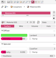
Specular color, specular intensity and hardness are properties of a material so we have also exposed the relevant panel to our custom renderer so that the user can set these values.

Code

The code changes needed in the inner shading loop of our ray tracer are limited:

if hit:
 diffuse_color = Vector((0.8, 0.8, 0.8))
 specular_color = Vector((0.2, 0.2, 0.2))
 mat_slots = ob.material_slots
 hardness = 0
 if len(mat_slots):
  diffuse_color = mat_slots[0].material.diffuse_color \
                    * mat_slots[0].material.diffuse_intensity
  specular_color = mat_slots[0].material.specular_color \
                    * mat_slots[0].material.specular_intensity
  hardness = mat_slots[0].material.specular_hardness

  ... identical code left out ...
  
  if not lhit:
   illumination = light * normal.dot(light_dir)/light_dist
   color += np.array(diffuse_color) * illumination
   if hardness > 0:  # phong reflection model
    half = (light_dir - dir).normalized()
    reflection = light * half.dot(normal) ** hardness
    color += np.array(specular_color) * reflection

We set reasonable defaults (line 2 - 5), override those defaults if we have a material on this object (line 6 - 11) and then, if we are not in the shadow, calculate the diffuse component of the lighting as before (line 16 - 17) and the finally add a specular component (line 18 - 21)

For the specular component we use the Phong model (or actually the Blinn-Phong model). This means we look at the angle between the normal (shown in light blue in the image below) and the half way vector (in dark blue). The smaller the angle the tighter the highlight. The tightness is controlled by the hardness: we raise the cosine of the angle (which is what the dot product is that we compute in line 20) to the power of this hardness. Note that the half way vector is the normalized vector that points exactly in between the direction of the light and the camera as seen from the point being shaded. That is why we have a minus sign rather than a plus sign in line 19 because dir in our code points from the camera towards the point being shaded.

Code availability

The code is available on GitHub.

Raytracing concepts and code, part 5, diffuse color

This is an article in a multipart series on the concepts of ray tracing. I am not sure where this will lead but I am open to suggestions. We will be creating code that will run inside Blender. Blender has ray tracing renderers of course but that is not the point: by reusing Python libraries and Blender's scene building capabilities we can concentrate on true ray tracing issues like shader models, lighting, etc.
I generally present stuff in a back-to-front manner: first an article with some (well commented) code and images of the results, then one or more articles discussing the concepts. The idea is that this encourages you to experiment and have a look at the code yourself before being introduced to theory. How well this works out we will see :-)

So far the series consists of the several articles labeled ray tracing concepts

Our rendered scene so far mainly consists of fifty shades of gray and that might be exciting enough for some but it would be better if we could spice it up with some color.

For this we will use the diffuse color of the first material slot of an object (if any). The code so far needs very little change to make this happen:

            # the default background is black for now
            color = np.zeros(3)
            if hit:
                # the get the diffuse color of the object we hit
                diffuse_color = Vector((0.8, 0.8, 0.8))
                mat_slots = ob.material_slots
                if len(mat_slots):
                    diffuse_color = mat_slots[0].material.diffuse_color
                        
                color = np.zeros(3)
                light = np.ones(3) * intensity  # light color is white
                for lamp in lamps:
                    # for every lamp determine the direction and distance
                    light_vec = lamp.location - loc
                    light_dist = light_vec.length_squared
                    light_dir = light_vec.normalized()
                    
                    # cast a ray in the direction of the light starting
                    # at the original hit location
                    lhit, lloc, lnormal, lindex, lob, lmat = scene.ray_cast(loc+light_dir*eps, light_dir)
                    
                    # if we hit something we are in the shadow of the light
                    if not lhit:
                        # otherwise we add the distance attenuated intensity
                        # we calculate diffuse reflectance with a pure 
                        # lambertian model
                        # https://en.wikipedia.org/wiki/Lambertian_reflectance
                        color += diffuse_color * intensity * normal.dot(light_dir)/light_dist
            buf[y,x,0:3] = color

In lines 5-8 we check if there is at least one material slot on the object we hit and get its diffuse color. If there is no associated material we keep a default light grey color.
This diffuse color is what we use in line 28 if we are not in the shadow.

Code availability

The code is available on GitHub.

Raytracing: concepts and code, part 4, the active camera

This is an article in a multipart series on the concepts of ray tracing. I am not sure where this will lead but I am open to suggestions. We will be creating code that will run inside Blender. Blender has ray tracing renderers of course but that is not the point: by reusing Python libraries and Blender's scene building capabilities we can concentrate on true ray tracing issues like shader models, lighting, etc.
I generally present stuff in a back-to-front manner: first an article with some (well commented) code and images of the results, then one or more articles discussing the concepts. The idea is that this encourages you to experiment and have a look at the code yourself before being introduced to theory. How well this works out we will see :-)

So far the series consists of the several articles labeled ray tracing concepts

In a further bit of code cleanup we'd like to get rid of the hardcoded camera position and look at direction by using the location of the active camera in the scene together with its rotation.
Fortunately very little code has to change to make this happen in our render method:

    # the location and orientation of the active camera
    origin = scene.camera.location
    rotation = scene.camera.rotation_euler

Using the rotation we can first create the camera ray as if it originated in the default -Z direction and then simply rotate it using the camera location:

    aspectratio = height/width
    # loop over all pixels once (no multisampling)
    for y in range(height):
        yscreen = ((y-(height/2))/height) * aspectratio
        for x in range(width):
            xscreen = (x-(width/2))/width
            # align the look_at direction
            dir = Vector((xscreen, yscreen, -1))
            dir.rotate(rotation)

Later we might even adapt this code to take into account the field of vision, but for now at least we can position and aim the active camera in the scene any way we like.

Code availability

The code is available on GitHub.

Raytracing: concepts and code, part 3, a render engine

This is an article in a multipart series on the concepts of ray tracing. I am not sure where this will lead but I am open to suggestions. We will be creating code that will run inside Blender. Blender has ray tracing renderers of course but that is not the point: by reusing Python libraries and Blender's scene building capabilities we can concentrate on true ray tracing issues like shader models, lighting, etc.
I generally present stuff in a back-to-front manner: first an article with some (well commented) code and images of the results, then one or more articles discussing the concepts. The idea is that this encourages you to experiment and have a look at the code yourself before being introduced to theory. How well this works out we will see :-)

So far the series consists of the several articles labeled ray tracing concepts

The code presented in the first article of this series was a bit of a hack: running from the text editor and lots of built-in assumptions is not the way to go so lets refactor this in a proper render engine that will be available alongside Blender's built-in renderers:

A RenderEngine

All we really have to do is to derive a class from Blender's RenderEngine class and register it.The class should provide a single method render() that takes a Scene parameter and returns a buffer with RGBA pixel values.

class CustomRenderEngine(bpy.types.RenderEngine):
    bl_idname = "ray_tracer"
    bl_label = "Ray Tracing Concepts Renderer"
    bl_use_preview = True

    def render(self, scene):
        scale = scene.render.resolution_percentage / 100.0
        self.size_x = int(scene.render.resolution_x * scale)
        self.size_y = int(scene.render.resolution_y * scale)

        if self.is_preview:  # we might differentiate later
            pass             # for now ignore completely
        else:
            self.render_scene(scene)

    def render_scene(self, scene):
        buf = ray_trace(scene, self.size_x, self.size_y)
        buf.shape = -1,4

        # Here we write the pixel values to the RenderResult
        result = self.begin_result(0, 0, self.size_x, self.size_y)
        layer = result.layers[0].passes["Combined"]
        layer.rect = buf.tolist()
        self.end_result(result)

Option panels

For a custom render engine all panels in the render and material options will be hidden by default. This makes sense because not all render engines use the same options. We are interested in just the dimensions of the image we have to render and the diffuse color of any material so we explicitly add our render engine to the list of COMPAT_ENGINES in each of those panels, along with the basic render buttons and material slot list.

def register():
    bpy.utils.register_module(__name__)
    from bl_ui import (
            properties_render,
            properties_material,
            )
    properties_render.RENDER_PT_render.COMPAT_ENGINES.add(CustomRenderEngine.bl_idname)
    properties_render.RENDER_PT_dimensions.COMPAT_ENGINES.add(CustomRenderEngine.bl_idname)
    properties_material.MATERIAL_PT_context_material.COMPAT_ENGINES.add(CustomRenderEngine.bl_idname)
    properties_material.MATERIAL_PT_diffuse.COMPAT_ENGINES.add(CustomRenderEngine.bl_idname)

def unregister():
    bpy.utils.unregister_module(__name__)
    from bl_ui import (
            properties_render,
            properties_material,
            )
    properties_render.RENDER_PT_render.COMPAT_ENGINES.remove(CustomRenderEngine.bl_idname)
    properties_render.RENDER_PT_dimensions.COMPAT_ENGINES.remove(CustomRenderEngine.bl_idname)
    properties_material.MATERIAL_PT_context_material.COMPAT_ENGINES.remove(CustomRenderEngine.bl_idname)
    properties_material.MATERIAL_PT_diffuse.COMPAT_ENGINES.remove(CustomRenderEngine.bl_idname)

reusing the ray tracing code

Our previous ray tracing code is adapted to use the height and width arguments instead of arbitrary constants:

def ray_trace(scene, width, height):     

    lamps = [ob for ob in scene.objects if ob.type == 'LAMP']

    intensity = 10  # intensity for all lamps
    eps = 1e-5      # small offset to prevent self intersection for secondary rays

    # create a buffer to store the calculated intensities
    buf = np.ones(width*height*4)
    buf.shape = height,width,4

    # the location of our virtual camera (we do NOT use any camera that might be present)
    origin = (8,0,0)

    aspectratio = height/width
    # loop over all pixels once (no multisampling)
    for y in range(height):
        yscreen = ((y-(height/2))/height) * aspectratio
        for x in range(width):
            xscreen = (x-(width/2))/width
            # get the direction. camera points in -x direction, FOV = approx asin(1/8) = 7 degrees
            dir = (-1, xscreen, yscreen)
            
            # cast a ray into the scene
            
            ... indentical code omitted ...

    return buf

Code availability

The code is available on GitHub. Remember that any test scene should be visible from an virtual camera located at (8,0,0) pointing in the -x direction. The actual camera is ignored for now.

Rayleigh scattering in Cycles

Prompted by a question in a comment by Joakim Poromaa Helger I came up with this approach to emulate Rayleigh scattering (the effect that turns the sky blue and the sun red at the same time) in Cycles: by combining a transparent and a glass shader.

In the picture above there is a bright white sun on the right. In a material that exhibits Rayleigh scattering (like air) blue light is scattered more than red light. That means that light traveling from a lightsource through such material will be tinted red because blue light is scattered to all sides. In a direction away from the direct path of the light we see just this scattered blue light and not (or much less) the direct light.

Now if we combine a red(ish) transparent shader with a blue(ish) glass shader, the transparent shader will cause some of the light to be passed through the object without regard for index of refraction and give it a redish hue, while the glass shader will pass some (refracted) blue light through and reflect some. (In the sample picture I have turned off caustics because that takes forever to give a good quality render but also because in this setup caustics exhibit a blue color while it should be redish as well). The node setup looks like this:

With some extra trickery we can correct the color for any caustics as well:

(Note that this image took 10,000 samples and the caustics are still very noisy. Clearly caustics is not Cycles strong point. The light/shadow inside the orb are due to the fact I placed it slightly below the ground but am to lazy to fix it).

We achive the caustic coloring by arranging that the camera sees the blue glass shader while any object receiving diffuse light (like the floor) sees a red glass shader, a distinction we can make with help of the light path node:

Now obiously the effect here is exagerated for demonstration purposes and arguably it is not a real simulation of Rayleigh scattering but for artistic purposes this might be a good start.

An X-Ray shader for OSL using an edge detection node

In this attempt to create an X-ray shader that highlights object edges we profit form the built-in facilities of OSL to compute derivatives.

The X-ray effect in the picture is mostly achieved by letting the meshes emit some light but more from their contours as seen from the camera.

(note that with all that transparency we need an awfull lot of samples to get a noise free result: even with 500 samples there is still noise visible in the image)

In order to determine what the contours are, we make use of OSLs built-in functions Dx() and Dy() that compute the derivatives of a function. The idea is that the derivatives for the current shading possition as seen from the camera change fastest at the contours of objects. This of course will only work reasonably well for curved objects. In the picture below we have a simple diffuse that is red when the sum of the derivatives is large. The small cube on the left has sharp edges that case an abrupt change that we cannot capture this way. The cube on the right has a bevel and a subsurface modifier added and does show edges.

shader der(
    point Pos = P,
    output vector dx  =0,
    output vector dy  =0,
    output float Lx = 0,
    output float Ly = 0,
    output float R = 0
){
    dx = Dx(Pos);
    dy = Dy(Pos);
    Lx= length(dx);
    Ly= length(dy);
    R = Lx + Ly;  
}

Sample node setup

The x-ray image at the beginning of this post was created with the following node setup:

Beside a mix of shaders the most important part is the texture coordinate that we take as input: Camera space is selected here. The add and multiplication nodes are there just to give us some control over the noise we want to mix in.

How to set up simple hdri environment lighting in Blender Cycles

In quite a few articles on this blog I present example images that use environment lighting and a detailed backplate. I found it not very intuitive at first to set up a scene in a way that gave me some control so I thought I'd share my findings here.

When using environment lighting with backplates you need of course have access to good resources and one of the best free resources I found is the sIBL Archive on hdrlabs.com. Each archive contains normally three images: a high resolution backplate, a low resolution hdri environment map and a high resolution hdri reflection map, all in a format that can be used by Blender directly. Just make sure you use an Environment Texture node (not a regular imaged texture). The environments we use here are all equilateral but Blender also has the option to use mirror ball images.

A high resolution (8000 x 4000 pixels) backplate is already huge and an hdri image is even bigger (typically 4 to 10 times) both because it uses more bits to store the information in each color channel and because it appears to compress less well. It would be wasteful to keep all this in memory if you don't need it because memory already is a precious commodity when rendering. Therefore each map has a different resolution: the backplate is very detailed, but is plain rgb, not hdri, and the environment map is very low resolution since you won't see it directly and lights don't need fine detail. In reflections however you might need some detail (if you have very shiny surfaces where you can see the environment) and in that case you might want to use the medium resolution reflection maps. In the image at the start of the article I used the low resolution enviroment map and as you can see the very glossy monkey on the right doesn't show a recognizable image in the reflection. In the image below we used a medium resolution reflection map which gives fair result while still being much smaller than an hdri map with the same resoltion as the back plate would be.

If we can see the background we have to create a setup for the world material nodes where we couple the highly detailed background image to the lower resolution environment or reflection map, in such a way that when we look a the background directly we see the backplate while in all other cases (like diffuse and specular reflection bounces for example) we use the hdri map. This is possible by using Cycles' light path node.

The light path node has an Is Camera Ray socket that will have a value of one if we are dealing with a camera ray and is zero otherwise. A camera ray is a ray that shoots directly from the camera so if our background is hit by a camera ray we present the high res backplate and in all other cases we present the hdri environment map. This is done by drivin the mix shader in the node setup above by this camera ray. Note that the backplate shader is the one that plugs into the lower input socket of the mix shader.

When you create your scene it is convenient to place your camera in the center, i.e. at location 0,0,0 because these environment images are shot like a panorama with the real world camera in its center. This doesn't have to be exact but in indoor scenes some distortion might be noticeable if you rotate the camera while it is not in the center.

Now if you want to change your view and lighting you could rotate the camera but then you would need to move all other objects as well. It might be much more convenient to rotate the background imagery. The backplate and the environment map will have to be linked of course to keep what you see and how things are lit in sync and the easiest way to do that is shown in the node setup below

The generated coordinates are fed through a vector mapping node before being connected to both background shaders. We now can rotate both images at the same time by changing the z-rotation value of the mapping node. (The other roatations are generally less useful as in these good quality pictures there is hardly ever the need to correct a tilted horizon for example but if need this could be done by rotating around the x or y axis).